


 nueva página del texto (beta)
 Inglés (pdf)
 Artículo en XML
 Referencias del artículo
 Enviar artículo por email
 Citado por SciELO
  Similares en
SciELO
Similares en
SciELO 
 Permalink
Nomenclature
| CADD | Computer-assisted drug design |
| DIFAC | Diseño de fármacos asistido por computadora |
| GABA | Gamma-aminobutyric acid |
| GABAA | Gamma-aminobutyric acid type A receptor |
| RMSD | Root-mean-square deviation |
| ΔG | Difference in Gibbs free energy |
| Δ8THC | Delta-8-tetrahydrocannabinol |
| UAM | Universidad Autónoma Metropolitana |
Introduction
Molecular docking simulations are powerful computational tools in the drug discovery and design fields. They play a fundamental role in predicting binding interactions between ligands and their target proteins, which contributes to the development of new therapeutic agents [1]. With the increasing need for efficient drug development strategies, molecular docking has become a frontline technique that accelerates the process of identifying potential drug candidates significantly [2]. In recent decades, advances in computational algorithms, increased processing power, and the availability of high-resolution structural data have enhanced the field of molecular docking. This has allowed us to explore a vast chemical space and evaluate thousands of compounds for their potential to bind to specific sites on proteins. By simulating the binding process, molecular docking gives useful details about the type of interaction, the binding affinity, and the specificity of ligands toward their target proteins [3].
Molecular docking is a structure-based method that typically implements an algorithm to explore the conformational space and a scoring function that predicts the affinity in numeric terms [4,5]. This combination is capable of search and predict the most favorable ligand positions in the binding site of interest [6]. There are several techniques for searching the ligand conformational space, ranging from random generation of poses to deterministic approaches [6-8]. To evaluate each generated conformation or pose and compare it with the others, scoring functions have been created. There are at least three types of scoring functions, namely: force field, empirically based and knowledge based. Force field types simplify the calculations by adding the ligand-protein interaction energy and the ligand internal energy. [4]. This is achieved by estimating electrostatic interaction values of the ligand-protein system such as hydrogen bonds and geometric variables such as ideal distances and angles. The terms used are calculated making use of equations such Lennard-Jones potential function or applications of the Coulomb's law [9]. The second type of scoring functions, the empirical ones, have several terms fitted by regression analysis of experimental binding energy data, although many parameters are estimated trough equations in a similar way than the force field types. The third type presents an interesting approach as it prioritizes the analysis of experimentally solved ligand- protein complexes to generate a score value based on the similarity of interactions [4,10], this based on the statistical premise that favorable interactions occur more frequently than unfavorable ones [5].
Broadly speaking, the molecular docking procedure consists of 4 steps: target and ligand selection, molecule preparation, molecular docking simulations and analysis of results. Of course, each of the steps requires the researcher's attention to make crucial decisions to obtain relevant results. The selection of both proteins and ligands can be based on results of experiments in biological models that point to probable ligand-protein interactions or from predictive models based even on machine learning. As for the preparation of the molecules, it is generally required to choose crystallographic structures of the targets with good resolution, without mutations, coming from species relevant for the objectives and without missing amino acid residues. The target must be prepared for the docking simulations by vacating the crystallographic ligands, usually eliminating water molecules and free ions, adding hydrogens, modelling missing amino acid residues and checking the protonation state of the latter. Ligands should be prepared by checking their protonation state at the relevant pH and it is advisable to perform geometry optimizations using force fields appropriate for small organic molecules. Thus molecular docking preparation has particularities regarding the software being used, but in general also it is required to specify the spatial center and the size of the simulation box. Once the results have been generated, it is the researcher's responsibility to evaluate their biological relevance and, if necessary, carry out re-docking validations.
The researcher should consider that the quality of the results of molecular docking simulations depends on the preparation and an adequate choice of parameters. Thus, particular attention must be paid when adding hydrogens to both ligands and receptors so that they realistically represent the protonation states at the natural pH of the ligand-protein environment to be simulated (usually pH 7.4). Histidine residues are difficult to represent [11] and may even represent a challenge to automate the simulation of their protonation states. Mutations in the amino acid sequence of the PDB crystal can lead to erroneous interpretations of results as they can greatly influence the specificity of ligand binding. It has also been found that the assignment of an adequate simulation box size can influence the quality of the results as suggested by a study [12]. On the other hand, it is also important to verify the completeness of the amino acid chain to be modeled in case gaps are found near the binding site of interest.
Recently, studies have been conducted in which molecular docking, in combination with other computational methodologies and including experimental validation, has proven to be a valuable tool in drug development. In this way, promising candidates have been found as anticancer drugs in which molecular docking has been used as a virtual screening tool [13-15]. In other studies, it has been combined with molecular dynamics simulations or other purely computational methodologies [16-18]. Although the field of cancer research is very broad, molecular docking has been used to contribute to the development of drugs in many other diseases such as diabetes [19], Alzheimer [20], autoimmune disorders, drug addiction [21,22] rheumatoid arthritis and osteoarthritis [22] among many others.
Regarding purely computational results, it is worth emphasizing that rigorous protocols must be followed, observing good practices as part of computer-assisted drug development. One of them is the necessary accompaniment of experimental validations, so molecular docking studies should not be taken as final results but as starting points. The relative ease with which molecular docking results can be obtained could lead to exaggerated optimism, so a critical mind must be maintained regarding the results and of course validate them experimentally, as recommended by Gentile and his collaborators [23].
It is important for the “novice” researchers beginning to work in the field of computer-assisted drug development to become familiar with the underlying theory of computational methodologies so that they can play a critical role in the development and outcome of their studies. The incorporation of artificial intelligence-based approaches can lead to obtaining results through “black boxes” whose inner workings we cannot understand but which can still produce valuable results. However, the researcher must assume the burden of making decisions based on rational judgment, free from exaggerated expectations or a naive perception of computational methods [24].
One of the main advantages of molecular docking is its ability to guide the rational design of new drugs. By identifying the most favorable binding conformations and providing a quantitative assessment of affinities, researchers can prioritize compounds with the greatest potential for therapeutic efficacy. Researchers can use this information to improve lead molecules, which might be able to treat diseases, by changing the chemical structure of the ligands to make them more selective, have better affinity, and work better with other chemicals [25]. Molecular docking is useful for more than just finding new drugs. It is also used in other areas of biological research, like studying how proteins and ligands interact and how existing drugs work, as well as looking at how a drug might be repositioned [3]. The biological relevance of the results of any molecular simulation study depends on many factors, ranging from the particularities of each simulation program to the criteria applied by each researcher [26]. Therefore, we must verify these results through in vivo and in vitro studies.
It should not be overlooked that this technique, while extremely useful, also has drawbacks and there are ongoing challenges to its improvement. One of the main drawbacks of the technique is the great reductionism and simplification of a process as complex as the formation of the protein-ligand complex. Molecular docking requires rigid structures mainly in the target, when we know that in nature proteins are extremely dynamic. The calculation of binding energies is also considered to be one of the main limitations while there is no combination of search algorithm and scoring function that combines speed and accuracy [5].
Currently, there is a wide range of software (Table 1) that is responsible for carrying out virtual screening and molecular docking processes; many of them require the purchase of a license and do not grant access to the source code. Fortunately, some software, like AutoDock Tools [27] and Racoon [28], is freely available and open source. However, there is no free software package that handles the entire molecular docking process. The closest approaches to this are online services, such as 1-Click Docking, which has a limited library of around 10,000 protein targets and is based on AutoDock Vina. This service offers the possibility of working with any protein model if the user uploads the file to the server, however, this functionality is behind a paywall. Another example of this type of service is SwissDock (free), which bases its operation on the EADock software. According to the authors, its success rate is comparable to AutoDock [29,9]. Like the latter, EADock bases its simulations on a force field (CHARMM) and a conformational space search algorithm with evolutionary characteristics. Interestingly, the SwissDock service's focus, as well as our motivation, is to make available to researchers and students a tool not aimed at experts in molecular modeling or computer science. SwissDock does not provide a straightforward method for conducting virtual screenings; despite the potential for exploiting the page's command-line access, the online site itself cautions about the service's instability. HADDOCK offers the online ability to run simultaneous docking of up to six molecules supporting proteins, small molecules and nucleic acids. Interestingly the HADDOCK protocol can be run locally but is limited to UNIX based systems and requires some user expertise as well as access to considerable computational power [30]. Another example is the HDOCK web service which supports only protein-protein and protein-DNA/RNA docking jobs [31]. HDOCK lite can be purchased for local execution free of charge upon completion of a form, although the source code is not explicitly provided. RosettaDock also offers a specific online service for protein-protein interactions which is easy to use but is limited to online use and a limited three-dimensional space due to its high computational power requirements [32]. There are several other servers with advantages and limitations which will not be reviewed in this paper as this is not one of our objectives.
The main disadvantage of online tools is that many of them do not offer the possibility of working with the same protocol on a local machine, although some of them allow running inferior versions with local computing resources. In addition, the researcher depends on an internet connection and access to these services is limited in the short term to the maintenance of the servers and in the long term to the survival of these due to funding reasons or other challenges.
AutoDock Tools is the ecosystem that integrates AutoDock and all the necessary tools prior to docking and includes the needed tools for the subsequent analysis of the results. The user can access the Python-written source code through this software. From a rigorous point of view, AutoDock Tools has all the functionalities to run molecular docking (but not virtual screening), and in theory, no external program is required for preparations or results analysis. However, from a pragmatic point of view and based on our experience, it is usually more advisable to execute certain procedures through other programs. Thus, in our laboratory, we prefer to use Chimera for manual trimming of crystallographic structures and clearing binding sites, or Discovery Studio and PyMOL for result analysis. In our opinion, AutoDock Tools has an unintuitive style of menu presentation. Additionally, we have experienced software instability in the form of error messages and unexplained fatal errors in the creation of simulation configuration files. Of course, these errors have a computer explanation but are not intuitive or user attributable.
The alternative option for running molecular docking simulations with a virtual screening approach is AutoDockVS Racoon, which is the work of the same team that created AutoDock Tools. It is a package that is distributed together with AutoDock Tools, so it is also open source and free. Racoon offers the ability to run many molecular docking simulations to search for the best ligand-protein candidates. There are currently two versions of Racoon, and each one provides notable advantages and disadvantages. The first version, simply called Racoon, is software that runs mass docking simulations on a local computer, although it also offers the possibility of working with Linux clusters. According to the authors [28], Racoon can assume automation of the separation of MOL2 models into individual ligands, work with ligand libraries, convert of molecules to PDBQT format (a mandatory format for docking), filter ligands, work with flexible residues, and automatically create reusable configuration files for simulations. Each docking simulation generates numerous individual files, necessitating the creation of custom computer code to filter the candidates or import the result files into AutoDock Tools.
On the other hand, the alternative version (Racoon 2) adds the possibility of analyzing the results of virtual screening within the same program using a robust filtering system. This version's current state of development removes the ability to work with a machine in a local environment, which is a disadvantage. This requires the creation of Linux clusters or local virtual machines to be able to exploit the workstation's computing resources. In either case, these requirements necessitate computing competencies that are beyond the skills or interests of most researchers specializing in laboratory work. Another relevant limitation is that this version only allows working with AutoDock Vina, to the detriment of AutoDock4.
In our laboratory work environment and molecular docking workshops, we have observed a significant portion of the community resisting the adoption of technical knowledge, not theoretical, related to molecular docking simulations. Working with them entails, for convenience and necessity, learning several computer programs with complementary functionalities. In our research environment, biological or chemical aspects, which are related topics, do not make up much of the necessary knowledge. For this reason, we seek to implement an “ask and forget” philosophy in which researchers and students can benefit from the advantages of bioinformatics without having to invest part of their research time in learning numerous computer programs.
To put this philosophy into practice in the use of molecular docking and virtual screening methods, we considered making a simple but reliable tool that would handle the whole molecular docking process and give away the source code and program for free. In this way, we propose a simple and improvable tool for perpetual access with local computational resources. When facing virtual screenings with large libraries of ligands and target proteins, a tool with these characteristics would save valuable research time and, of course, would also save the investment of monetary resources from the budget in subscription plans for online services. On the other hand, this program could serve as an academic resource, helping biological sciences students overcome their aversion to this type of method due to its technological advantages.
Based on existing molecular docking tools, we designed a set of mutually coherent computer programs to speed up work with numerous ligands and target proteins, simplify simulations, and make these techniques easier to understand for researchers with limited computer science training. We conceived of the tool as open source that is both free and easy to use. Currently available virtual screening and molecular docking simulation programs require researchers to make numerous configurations and navigate unintuitive menus. This is usually not attractive to scientists or students specializing in laboratory work, and it interposes a significant learning curve. Furthermore, one of the objectives was to develop a robust format for presenting results, conceptualized as a massive report of rows and columns. This approach aims to simplify the filtering, discrimination, and interpretation of the large amount of data obtained. The present work aimed to create an automated computational tool that could perform multiple simultaneous studies of molecular docking. This tool would automatically prepare ligands and target proteins for the autodock4 molecular docking simulation procedure. It would also make configuration files for each molecular docking simulation, run the preparation steps for the docking site and the molecular docking processes at the same time, and make and create huge reports with the detailed results of the simulations. The tool also allows the expert user to manipulate critical parameters and preparations to obtain valuable predictions, benefiting from numerous automations.
Table 1 Some popular docking software and tools.
| Software | Distribution | Open source | Automated/Easy to use | Ref. |
|---|---|---|---|---|
| DOCK 3.7 | Free for academic use | Yes | No | [42] |
| Glide | Commercial | No | Yes | [43] |
| AutoDock | Free | Yes | No | [9] |
| Arguslab | Free | Yes | No | [44,45] |
| MolDock | Commercial | Pseudo-code released | No | [46] |
| Vina | Free | Yes | No | [47] |
| GOLD | Commercial | No | Yes | [48] |
| EasyDock | Free | Yes | Yes | [49] |
Material and methods
The tool described here was designed as a set of specialized modules that allow the entire molecular docking simulation process to be automated and carried out in a massive way. The summarized function of each module can be found in Table 2 and the workflow can be consulted in Fig. 1. As the source code was being worked on, many tests of the code's partial operation were run using random molecules. To prove that the tool worked, the final test of unified operation was done with cannabinoids in active sites of GABAA receptor. The tool does not include a graphical interface, so it was designed to run in interactive console mode (Supplementary Data 1). All the modules in this tool were written in Python and prepared to run on Windows operating systems capable of running Python 3.11. The tool was developed with the help of Visual Studio Code, a code editor.
Software created by other entities was used for this project. Simulations were conducted using the autodock4 and autogrid4 command lines. The OpenBabel command line was used to make the ligand molecules smaller in geometry. Two AutoDock tools modules were modified for this project to change the ligands and proteins to pdbqt format Fig. 1. To test how well the tool worked with different GABAA receptor structures, docking simulations of nine cannabinoids were used. The cannabinoids used were Δ8-tetrahydrocannabinol (Δ8-THC), cannabigerol, cannabichromene, cannabidiol, cannabinodiol, cannabielsoin, cannabicyclol, cannabinol, and cannabitriol, whose 3D models were obtained from the PubChem website. 11 structures were used for the tests, which corresponded to the Protein Data Bank codes 6X3W, 6X3X, 6X3T, 6X3U, 6X3V, 6X3Z, 8DD2, 8DD3, 6X40, 6X3S, and 6I53.
Furthermore, the 3ILZ PDB structure was only used to test the normalization of the different atom locations; docking simulations were not run on it. Docking simulations with GABA and diazepam ligands were also run in the 6X3X structure. This is to verify the tool's predictive capacity with respect to the same ligands that this structure includes. Simulations were conducted on a desktop computer with an AMD Ryzen 5 7600X 6-core processor, 12 logic processors overclocked at 5400 Mhz under Windows 11 operating system with 32 GB of RAM installed. Docking simulations run with UAM-Ixachi were performed by allowing the program to be as automated as possible. The docking results described here are reproducible under the specified conditions (approximately, due to the implicit generation of random seeds for the simulations) by following our procedure and the user guide available in the public repository. We created a new UAM-Ixachi project and created a plain text file containing the PDB IDs mentioned above, and created a folder with cannabinoid, GABA, and diazepam ligands in sdf format to then provide to UAM-Ixachi. The program was set to use 12 logical processors, and the box size was standardized to 18.75 Å on each axis (50 points with 0.375 Å spacing). Each docking simulation was repeated 100 times with a moderate exhaustiveness of 2,500,000 energy evaluations. Once UAM-Ixachi created the docking specification file, we edited it using Excel: We filtered out all GABA and diazepam docking simulations and disabled them except for the binding sites of the PDB structure 6X3X. After approximately 23 hours UAM-Ixachi notified the completion of all procedures. We opened the bulk H-bond report and filtered the results by cluster size and predicted binding energy, the frequency of occurrence of H-bonds with specific amino acid residues was obtained with the Excel “COUNTIF” formula. The graphical representation was obtained with Discovery Studio and Pymol with the file paths provided by the H-bond report.
https://1drv.ms/f/s!AiwrqGMGvesstXgOcz3Hn1Q2mfI9?e=903be7. Here, it is possible to consult, among other things, the raw versions of the hydrogen bond and cluster reports from all the docking simulations carried out in this work. In this address also was included a glossary with the fundamental concepts for understanding the design of the tool developed for this project.
The source of the structures used for molecular docking is the PDB standard, which is one of the formats with which protein structures are currently distributed. The computing basis for the simulations implemented here is autodock4, for which its creators designed the PDBQT format, which is a modification of the PDB format. To carry out the simulations, autodock4 is based on a genetic algorithm and a force field. Some of the defined concepts in the glossary are Protein Data Bank, PDB Format, Molecular Docking Simulation Tools, PDBQT Format, GPF Format, DPF Format, DLG Format, Hydrogen Bonds in Pharmacology, and Gibbs Free Energy.
The tool was designed to provide maximum convenience to both the expert user of molecular docking simulations and the novice user. To this end, the tool was programmed to manage individual projects requested by the user. In addition, considering the use of the tool with large sets of proteins and ligands, a convenient automatic system for assigning binding sites based on the coordinates of crystallographic ligands included in PDB structures was enabled. However, it was programmed to allow customization of the simulation center coordinates and the grid box size, as well as allowing the disabling of specific docking simulations in a simple manner. The tool was designed to facilitate the filtering of results, assuming that these will be presented in a huge amount of data. Many simulation parameters such as those related to the genetic algorithm were fixed, although the expert user can adjust these and other relevant parameters in an accessible configuration file.
Table 2 Synthesized description of the functions of each module. They are presented in the order in which they are executed.
| Module | Specialized function |
|---|---|
| Manager module (manager) | The administration of each module's execution. Interaction with the user. It unites all the specialized modules, executing them in the correct sequence. The manager was programmed to prompt the user for a directory with experimental ligands and a file with the list of PDB codes to use. It was also programmed to only ask the user about the simulation configuration once. This configuration includes the number of runs, completeness of each run, maximum number of processors to use, and grid size. Additionally, manager controls the base directory for the tool in C:\UAM-Ixachi\ to store each of the docking simulation-specific directories organized in project folders. Moreover, instructions were included to create the directory tree to store the molecules processed by the specialized modules in the directory named “MDSources” within the project folder. It was programmed to manage information provided by the user, as well as certain data generated by specialized modules, and store it in a user-editable configuration file at the path C:\UAM-Ixachi\Ixachi.cfg. |
| Download Module (pdb downloader) | The process involves downloading a list of structures from the Protein Data Bank. The system processes a list of PDB codes, each of which corresponds to a 3D protein structure. It was programmed to connect to the Protein Data Bank database, and then download and store the files in the “Raw_receptors” directory within “MDSources”. The code list must be created by the user in a plain text file. |
| Crystallographic structure cutter module (crystalcutter) | Each PDB structure is trimmed to separate crystallographic ligands. The module is specifically designed to process protein structures that have been downloaded using the pdbdownloader. The module was programmed to read PDB files and extract from the HETNAM section all the names of heterogeneous crystallographic components. The tool implemented automatic verification of CONECT records in PDB format. The logic for telling crystallographic ligands apart was based on the information in the PDB format guide (RCSB PDB, n.d.): if the CONECT section refers to atoms of compounds that are connected to different residues, then the compound was thought to be structural and would be saved in the same file as the protein. On the other hand, if CONECT records indicated only intramolecular bonds, this compound would be considered a free ligand. Additionally, the tool was designed to remove ions and water by default, rather than keeping them as separate files. The tool was designed to preserve and reuse crystallographic ligand files to ensure automatic grid center coordinates. Crystalcutter has instructions on how to make a very detailed log of the clipped residues in the file …\MDSources\Clipped_receptors\lig_id.log within the project folder to facilitate the diagnosis of failures in the identification of free ligands. |
| Alternative location atoms normalization module alternate location fixer | Consolidation of atoms with alternative locations. The tool was designed to identify ATOM records from the PDB format that refer to the same atom with alternative conformations and eliminate all except the one with the maximum occupancy value assigned according to the PDB format. It was also programmed to rewrite the serial numbering of each of the atoms after eliminating the alternative atoms. |
| PDBQT format conversion module (molprep) | The process involves converting proteins and ligands into the PDBQT format. It was designed to automate the preparation procedures for protein and ligand molecules. It was programmed to take any number of ligands (indicated by the user) in sdf or mol2 format, minimize their geometry with the MMFF94 force field, and then convert to pdbqt format, explicitly conserving only the polar hydrogens, adding Gasteiger charges, and specifying rotatable bonds; this was done through the Open Babel command line and the prepare_ligand4.py module, extracted from AutoDock tools. The latter were modified to enable and repair their operation within command lines. The user could ask the tool to work with any number of proteins, and change the format to rigid pdbqt format, adding polar hydrogens, and using the prepare_receptor4.py module from AutoDock tools to assign Gasteiger charges. |
| Docking simulations preparation module (multidock) | The directory tree for each docking simulation is
prepared. The first step of this module is to create the
specification file for the docking simulations. For this
purpose, the module records all the protein-ligand combinations
specified by the user and assigns binding sites automatically
based on the crystallographic ligands included in the PDB
structures. Once created, the module pauses to allow the user to
add or customize simulation boxes and fine-tune the protein and
ligand models prepared for the simulations. The process involves
creating configuration files for both autogrid4 and autodock4.
Performs multiple functions. One of them is to calculate the
center of the grid box for each active site to be evaluated.
Multidock was set up to find the center of the grid's z
coordinate by adding up all the z coordinates of the atoms in
each crystallographic ligand that was cut out by the
crystalcutter module and using the formula |
| Multiprocess module (grid_launch and dock_launch) | It was designed to launch several autogrid4 and autodock4 processes simultaneously, with a limit set by the user and only restricted by the number of logical cores or processors on the computer. To achieve this, the "Pool" multiprocessing tools included in Python 3.11 were implemented. |
| Results report module (succesreport and resultparser) | The task involves creating reports for both successful and unsuccessful simulations, as well as compiling data on all the clusters that emerged during the simulations. The system is designed to prepare a report in csv format that summarizes all the results of autodock4 simulations, identifying those that were successful and those that failed, and collects the cause of the failure. We programmed the reading of the last three lines of the dlg files containing the phrase identifying failure or success, in addition to the time taken by the simulation and the end time. The result parser module is responsible for parsing each autodock4 result that is presented in the form of .dlg files. It was programmed to check the final region of each file, where the dlg format stores the formed clusters. Then, it was set up to read the data about cluster size and minimum binding energy and combine it with data about ligands, sites, proteins, and access paths. Finally, it put all this information into a report in CSV format that can be opened in Excel and other spreadsheet programs. |
| H-bond report module (hbondanalyzer) | The report detailing the H-bridges formed in each
run, incorporating cluster data, is prepared. This is an
improvement of the resultparser module to include the amino acid
residues that form H-bonds with the ligands. First, we designed
the module to read the.dlg files to extract each conformation of
the ligand within a simulation into a separate file and name the
files with consecutive numbers within the directory created for
the specific ligand-site-protein simulation. This was achieved
by removing the “DOCKED:” header from the docked atomic
coordinates section, resulting in atomic assemblies capable of
generating molecules in PDBQT format. The next step was to open
each conformation file and measure the distance of each
experimental ligand atom to the protein atoms. To find H-bonds,
the following logic was programmed: if a ligand atom in a
certain configuration was at a distance of 3 Å or less from a
protein atom, and if one of them was identified as an H-bond
donor at the same time that the other was identified as an
H-bridge acceptor (according to the PDBQT format), then
information about the amino acid residue that the atom belongs
to is read. The tool was programmed to add this information to
the bulk report, along with all the data necessary to identify
the protein, ligand, site, conformation number, binding energy,
parent cluster, cluster size, and file paths. The distance
formula between two points was implemented to measure the
3-dimensional approach of the atoms participating in H bonds
implemented as |
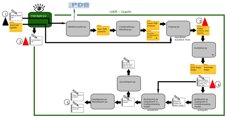
Fig. 1 UAM-Ixachi workflow. The grey rectangles represent the specialized python modules that make up the tool. The green rectangle represents the supervisor module. Below the modules are the tools or software developed by third parties that UAM-Ixachi uses. Red triangle mark steps where the expert user can optionally intervene. 1) The black triangle icon represents the only mandatory user interaction where the user provides to UAM-Ixachi with inputs (PDB ID list of proteins and ligands in mol2/sdf format) and simple settings. 2) The general configuration file is automatically generated but the expert user can change here relevant parameters such as the customized path of the "AutoDock Linear Free Energy Model Coefficients and Energetic Parameters" file, as well as those related to genetic algorithm and others. 3) UAM-Ixachi produces protein and ligand models in PDBQT format ready for molecular docking simulations, however as this is a crucial step the tool allows a pause for the expert user to provide his manually prepared models. 4) UAM-Ixachi also automatically generates protein-binding site-ligand pairings for docking simulations and assigns simulation box sizes and centers. Here the expert user can set custom box sizes and centers as well as disable unwanted simulation pairings. 5) The tool outputs are produced in the form of mass reports with .csv extension that are easy to analyze. * multidock.py uses the crystallographic ligands extracted by crystalcutter.py to automatically assign the center coordinates for each docking simulation.
Results
Protein structures automatic download
The specialized pdbdownloader module successfully processed the list containing PDB ID codes. All the requested structures were downloaded, except for 8DD3. This issue was investigated, and it was verified that the structure is not available in the database in PDB format.
Clearance of binding sites and stored crystallographic ligands
The specialized crystalcutter module appropriately identified the ligand molecules and discriminated between other molecules, such as structural carbohydrates, and non-standard amino acids. The cleaved crystallographic protein structures were individually checked for coherence with the original PDB structures. Each crystallographic ligand was not only removed from the structure, but the tool identified them and kept them in separate files, as expected, producing a total of 36 ligands files. Each file's consistency was verified individually, and its structural and chemical identity was verified with the original PDB structure. It was verified that all the structures conserved by the tool in the same protein model file corresponded to carbohydrates or non-standard amino acids, and separate files were not created for these, as expected. The integrity of the amino acid chains was adequately preserved. Figures 2 and 3 show a selection of these results.
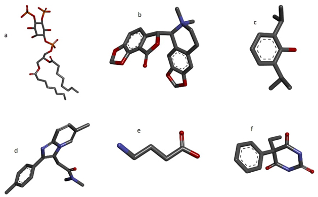
Fig. 2 Sample of 6 of a total of 36 crystallographic ligands isolated and automatically extracted by the crystalcutter module. (a) Dioctanoyl l-alpha-phosphatidyl-d-myo-inositol 4,5-diphosphate cleaved from the 6I53 structure, (b) (-)-bicuculline methochloride from the 6X3S structure c) Propofol cleaved from the 6X3T structure, (d) Zolpidem cleaved from 8DD2 structure, (e) GABA cleaved from the structure 6X3U, (f) Phenobarbital from the 6X3W structure.
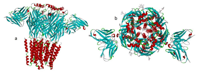
Fig. 3 Here are two out of a total of ten GABAA receptor models that have been automatically cropped by crystalcutter. (a) The 6X3X cropped structure; all binding sites were emptied by the tool. (b) The top image of the 8DD2 cropped structure shows the molecules that can be seen in the channel and the outside edges. These molecules are the structural carbohydrates that are maintained in the protein file.
Normalization of atoms with alternative locations
It was proven that the altlocationfixer module found atoms located in alternative places, identified different versions of the same atom, conserved the version of the atom with highest occupancy, removed the alternative marker in line with the PDB format, and serialized the atoms again (Fig. 4).
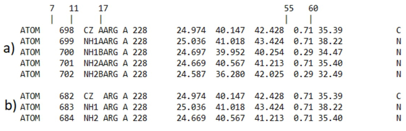
Fig. 4 Comparison of a 3-atom block in PDB format from the arginine residue 228 of the 3ILZ structure. The comparison is made between the block before and after processing using altlocationfixer. Columns 7 to 11 provide the serial number of the atom, column 17 indicates the name of the alternative location, and columns 55 to 60 indicate the occupancy value of each alternative location. (a) This block displays the atoms with alternate positions of the original PDB structure. The NH1 and NH2 atoms exhibit two distinct positions each, but the CZ atom is represented as a single entity. (b) The atoms block displays the outcome of automated processing using the altlocationfixer module, which detected atoms with alternative locations, eliminated those with lower occupancy, deleted the alternative location identification from column 17, and restored the serialization of the atoms.
Converting proteins and ligand models to PDBQT format
The ligand and protein molecules that came out of the molprep run were checked, and the rotatable bonds in the ligands were found to be consistent. It was verified that partial charge values were added, and the structure of the proteins and experimental ligand molecules was preserved. Crystallographic ligands did not require format conversion and were therefore retained in PDB format. It was confirmed that the hydrogens added to the proteins matched the amino acids' protonation states at pH 7.4. As expected, no non-polar hydrogens were found. The experimental ligands that were processed by the tool were shown to clearly conserve only polar hydrogens. The protonation states of the ligands were found to be consistent with a pH of 7.4.
Automatic preparation of docking simulations
The multidock module created 336 new directories, one for each docking simulation and named them in the intended format (they can be found in the online repository). Multidock automatically created 36 configuration files for creating atom-specific maps. The maps configured by multidock were the minimum amount needed for all 336 autodock4 simulations. Each one of the configuration files was automatically named by the tool according to the format to identify the grid's size and center. In the configuration file's internal data, the protein that corresponds to the configuration file was specified. As can be seen in Fig. 5, the grid centers automatically calculated by multidock turned out to be consistent with the region where the crystallographic ligands were in the original PDB structures. Additionally, multidock created all 336 *.dpf configuration files for autodock4 automatically, one for each protein-ligand-site docking simulation and saved them in their own separate directories. After verifying a sample of ten configuration files in dpf format, it was determined that the atom-specific maps had been correctly assigned in their internal data and were appropriate for each docking simulation. It was also verified that the rest of the parameters, such as the number of runs per simulation, completeness, etc., were correct.
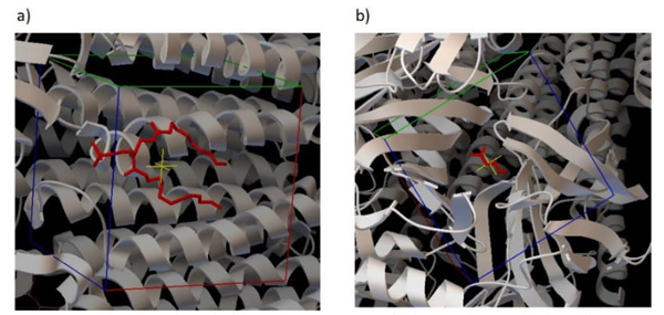
Fig. 5 Grid boxes generated by multidock. This is a sample of 2 out of a total of 36 binding sites. The protein structure is shown in a ribbon fashion, with crystallographic ligands indicated in red. The clear cube symbolizes the automated grid volume, with the center being denoted by a yellow cross. To depict it, it was rendered using AutoDock tools using the coordinates computed by multidock. (a) A grid was created for the 6I53 structure, with the center located at the coordinates (109.841, 130.663, 127.202). (b) This panel shows the grid box obtained by multidock for the 6X3U structure at the coordinates (113.143, 115.248, 153.214), specifically at a site involved in GABA binding.
Docking simulations in multiprocessing mode
The gridlaunch and docklaunch modules were executed in consecutive sequence in the respective order. Each module launched four simultaneous processes, as expected, according to the chosen configuration. In total, 36 autogrid4 processes and 336 autodock4 processes were executed. The 336 molecular docking simulations were completed in approximately 20 hours.
Failures in docking simulations
Success report generated a report with 336 rows corresponding to each of the docking simulations. No failed simulation was found in the report. Resultparser generated a report of 3279 rows corresponding to each of the clusters formed in all simulations, with all the data necessary to identify individual clusters.
Automated mass reporting of hydrogen bonds
The bulk report contains the results of all molecular docking simulations compiled by hbondanalyzer, which contains all the relevant data for the individual identification of each simulation run. The module made 33600 rows in the report, one for each run of the docking simulation, and identified 43878 hydrogen bonds between amino acid residues and ligands. Under the conditions described, the report took approximately 4 hours to complete.
Comparison of binding and ligand pose prediction tests
Here are the RMSD (heavy atoms) values for each cluster in the simulation. They show the difference between the crystallographic ligand and the best ligand configuration (based on ΔG). It was right that the simulations at the 6X3X structure predicted how GABA would be arranged at the known site in the extracellular domain, where the β2 and α1 subunits meet, with the carboxyl and amino groups facing the right direction. Docking simulations of GABA at the "ABU A 405" site were accurate (this site designation and all others used in this paper correspond to the original PDB structure ligand names). One cluster was obtained with 99 similar configurations and a RMSD value of 0.6 Å (the best simulated configuration vs. crystallographic pose). This, and all the results of the comparative simulations, can be consulted in Table 3. Fig. 6 shows the results in 3D configurations.
For the GABA docking simulations at the "ABU C 405" site, three clusters of 63, 21 and 16 configurations were obtained. The 63-member cluster showed an RMSD value of 0.7 Å of the best configuration (Fig. 6(b)).
At the "DZP A 406" site, docking simulations of diazepam resulted in one principal cluster made up of 99 configurations with an RMSD of 4.87 Å with respect to the crystallographic ligand. While in the crystallographic ligand, the chlorine atom pointed towards the helix of the β2 subunit, in the simulation result it pointed towards the cytosol. The oxygen in the crystallographic ligand's carbonyl group, on the other hand, pointed toward the α1 subunit and slightly toward the extracellular space. The simulation result pointed to the extracellular space (Fig. 6(c)). When diazepam was simulated at the "DZP C 406" site, a single cluster was found with 100 consistent configurations in the binding pocket. These configurations had different poses for the crystallographic ligand, though. On this occasion, the simulation placed the diazepam molecule in a position in which the carbonyl oxygen pointed in the direction of the channel, while the crystallographic ligand pointed to the α1 subunit (Fig. 6(d)). The cluster's representative RMSD value was 5.66 Å. For the simulations at the "DZP D 404" site, one principal cluster was identified. It had 99 diazepam configurations. The poses of this simulation turned out to be slightly similar in the cyclic groups, but the chlorine atom pointed in opposite directions. The representative RMSD was 3.77 Å. Fig. 6 shows this result in 3 dimensions. The docking simulation results for the "DZP E403" site showed a single cluster with 100 similar poses. In this simulation, the crystallographic pose was consistently reproduced with the arrangement of the groups in the correct manner. (Fig. 6(f)). The RMSD value was determined to be 0.85 Å with respect to the ligand's coordinates in the raw PDB structure.
Table 3 Synthesized outcomes of the tool's comparative docking simulations. Only results from simulations of the ligands occupying the same binding site as in the 6X3X structure are shown. The RMSD value refers to the cluster configuration that has the lowest ΔG.
| PDB site code | Location | Ligand | Cluster size x/100 | Identification Site | Pose Prediction | ΔG x̄ | RMSD |
|---|---|---|---|---|---|---|---|
| (kcal/mol) | (Å) | ||||||
| ABU_A_405 | Interface of β2 and α1 subunits. extracellular domain | GABA | 99 | Yes | Yes | -6.4 | 0.6 |
| ABU_C_405 | Extracellular domain between β2 and α1 subunits (chains C and D respectively) | GABA | 88 | Yes | Yes | -5.13 | 0.70 |
| DZP_A_406 | Transmembrane domain at the β2 and α1 interface | Diazepam | 99 | Yes | No | -8.63 | 4.87 |
| DZP_C_406 | Transmembrane domain at the β2 and α1 interface. | Diazepam | 100 | Yes | No | -8.58 | 5.66 |
| DZP_D_404 | Extracellular domain at the α1 and γ2 interface. | Diazepam | 99 | Yes | No | -8.23 | 3.77 |
| DZP_E_403 | Transmembrane domain between γ2 and β2 subunits | Diazepam | 100 | Yes | Yes | -8.28 | 0.85 |
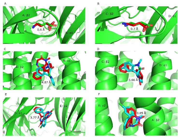
Fig. 6 Superposition of the ligands in the pose predicted by the simulations and the crystallographic poses. Comparative simulations were conducted to validate the tool using the 6X3X structure of the GABAA receptor. The viewpoint in all portions is oriented towards the extracellular space in the top half and towards the cytosol in the bottom part. Chain identifiers and subunit names are indicated over the protein structure. The root mean square deviation (RMSD) value is shown next to the molecular overlay. The hydrocarbon structure in red represents the ligand that was docked in the simulation. (A) and (B) demonstrate the relative degree to which GABA poses overlap in the extracellular domain. The comparison of diazepam in three benzodiazepine binding sites of the transmembrane domain is shown by (C), (D), and (F), (E) represents the degree of overlap between diazepam and the benzodiazepine site in the extracellular domain.
Cannabinoid docking simulations, filter the top 10 clusters
Of the 3279 clusters formed by all docking simulations, the 10 best were chosen
demonstratively (Table 4). To
discriminate the clusters we created a very simple scoring function:
Table 4 Top 10 clusters obtained from all cannabinoid simulations. Their ranking is based on the average Gibbs free energy and the cluster size.
| Cluster rank | Cluster size | ΔG x̄ | Receptor code | Ligand | Binding site code | H-bonds: Residue, Count |
|---|---|---|---|---|---|---|
| 1 | 99 | -10.2 | 8DD2 | Cannabinol | R5R_C_402 | THR 262, 99 |
| 2 | 100 | -9.53 | 6X3W | D8THC | UQA_C_501 | SER 270, 100 |
| 3 | 100 | -8.95 | 6X3X | Cannabicyclol | DZP_C_406 | ASN 265, 71 LEU 232, 29 |
| 4 | 91 | -9.68 | 6X3X | Cannabinol | DZP_E_403 | GLN 224, 51 SER 280, 61 THR 281, 33 |
| 5 | 98 | -8.84 | 6X3T | D8THC | PFL_D_601 | ILE 228, 97 LEU 232, 1 |
| 6 | 90 | -9.57 | 8DD2 | D8THC | R5R_D_601 | SER 205, 86 THR 142, 86 TYR 160, 86 |
| 7 | 98 | -8.76 | 6X3T | Cannabinol | PFL_B_601 | ILE 228, 98 |
| 8 | 98 | -8.75 | 6X3X | Cannabidiol | DZP_C_406 | ASN 265, 98* THR 262, 2 |
| 9 | 88 | -9.73 | 6X3X | Cannabicyclol | DZP_E_403 | GLN 224, 69 SER 280, 21 |
| 10 | 98 | -8.61 | 6X3W | Cannabinol | UQA_C_501 | LEU 223, 95 |
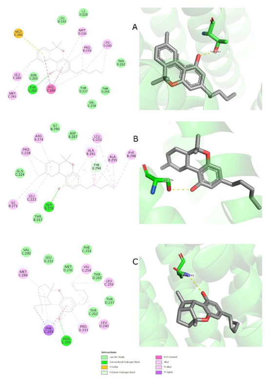
Fig. 7 Visual representation of the 2D and 3D interactions of the three most significant clusters that were created during the cannabinoids docking simulations at the GABAA receptor. All of them are located inside the benzodiazepine binding sites. The 3D models show hydrogen bonding, which are represented by dashed yellow lines. (A) Cannabinol forms a hydrogen bond with the threonine residue 262. (B) Δ8-THC forms a hydrogen bond with the serine residue 270. (C) Cannabicyclol can create a hydrogen bond with asparagine 265.
Discussion
UAM-Ixachi has been designed to increase accessibility for non-computer users by including scenario handler and error control code. This prevents the tool from freezing or terminating unexpectedly in subsequent steps. The tool also manages interaction with the user by verifying the requested grid size, number of runs, and processors. If the user's information is invalid, the program will indicate the correct format and request it again.
The tool can be executed for a complete process or individually for each specialized function module. For example, the user can run crystalcutter individually to crop PDB structures in masse. The manager module was created to address these needs by asking the user for all necessary information and reading and writing to the configuration file. The tests have shown that crystalcutter is a robust selector for cutting proteins in PDB format that includes ligands. Vacating binding sites in PDB structures with docked ligands is usually tedious using programs like Chimera or Discovery Studio, as it requires navigating through various menus and performing visual verifications on extensive 3-dimensional structures. Crystalcutter effectively isolated and stored crystallographic ligands and put them into files, preserving all component atoms and coordinates specified in the original PDB structures. All ligand-free proteins models have been verified to conserve their entire structure, including standard amino acids, non-standard amino acids, and structural carbohydrates (Fig. 2 and 3).
The crystalcutter module has been found to be effective to identifying free ligands, but it faces challenges when dealing with free and unitary crystallographic ligands with more than one residue designation, possibly causing a false negative identifying an object as a ligand. Also, the specification of hydrogen bonds in the CONECT section may cause the same problem. To address these issues, the code can be improved to track covalent bonds with standard amino acid residues and ignore CONECT records involving hydrogen atoms. Crystalcutter was programmed to remove water molecules and ions by default, which could be controversial due to their importance in docking simulations and their dynamic nature [1]. Programming a module that correctly configures amino acid protonation states is also challenging, as demonstrated by histidine residues with a dynamic protonation state [33] and even the official AutoDock tools guide warns users about hydrogen allocation, suggesting them to check ligands and target proteins using external programs before starting simulations [34]. For this, a pause and a warning were implemented in the tool here described so that users can check the proteins and ligands, if users choose to continue without modifications, simulations will be executed with automatic molecule preparations.
Altlocationfixer was created to address the issue of PDB structures including atoms with alternative locations. These models produced aberrations in the coordinate format when hydrogens bonded to atoms with alternative locations were added. Altlocationfixer solved this problem by producing structures in PDB format with single atom locations and converting them to pdbqt format using molprep. The PDB format established an atom serialization system [35] that was disturbed by the elimination of atoms with alternative locations and water molecules, ions, and crystallographic ligands. Serial number reassignment for each atom was implemented in altlocationfixer.
A problem generated by altlocationfixer was identified since the output format of the molecules processed by this module continues to be PDB. As mentioned above, altlocationfixer reconstructs the atomic serial numbers but leaves the CONECT records unchanged, making them useless. This only affects PDB files stored in the “clipped proteins” directory and should not pose any problems for the tool to function, but it is not recommended to reuse these models for other purposes. This problem can be resolved by improving the module code to normalize the CONECT records with the new serial numbers and adding annotations to the REMARK records to warn about the deletion of atoms with alternative locations.
Originally, it was planned to use the OpenBabel command line to convert large amounts of molecules to the pdbqt format. However, only some of this format's features worked, as demonstrated by the fact that rotatable bonds weren't always assigned to ligands correctly, and proteins lost some of their amino acid names. Because of this, it was finally decided to use the prepare_ligand4 and prepare_receptor4 modules from the AutoDock tools to make the conversion to pdbqt format. These modules are not prepared to work with absolute file paths, so they were modified so that they could be used within the molprep module script. To avoid instability in AutoDock tools, the modules were modified in the UAM-Ixachi directory, while the original modules were left intact in the AutoDock tools installation. These modules extracted from AutoDock tools import computational code from other AutoDock tools modules, and their authors designed them under Python 2, so they are not prepared to work autonomously. This requires, for the moment, a complete installation of AutoDock tools on the system on which the tool described here is intended to be run. In future versions of the tool, we will isolate the necessary code or generate new code to work with these conversions, eliminating the need for a full installation of AutoDock Tools.
The exclusive assignment of polar hydrogens was implemented in molprep, as the force field used by autodock4 was calibrated to work in this way [36].
Multidock results showed the module's robustness by generating all specific protein-ligand-site simulation directories, which were 336. This number is coherent because 9 experimental ligands were evaluated in 36 binding sites, and 12 simulations were executed with the tool in the PDB 6X3X GABAA receptor binding sites. Multidock was designed to identify and prepare the minimum number of autogrid4 processes, resulting in reduced computation time and disk space usage.
Multidock was used to automatically generate coordinates for the center of the grid in three-dimensional volume calculations for docking simulations. The grid box was determined based on crystallographic ligands cut by crystalcutter and user-specified data about the size desired. However, the idea of automatically calculating the grid size based on the size of the binding site was discarded due to variability in size and shape of protein cavities, as well as the challenge of identifying cavities as binding sites. The location of the binding site could also result in misleading size calculations. Some PDB files include SITE records that identify active sites, which could improve UAM-Ixachi code. The creation of a binding site identifier module remains as a perspective, as it has been implemented in other programs from a non-topological approach, such as EADock [29]. A simple approach we could use to complement the automation of the grid box is reported by Feinstein's research group in which they propose a grid box optimization based on the size of the experimental ligand, which can be implemented in future versions of our tool [12]. The tool was also considered to prepare blind docking simulations when PDB structures did not include crystallographic ligands but was discarded due to the tool's design for mass simulation studies and the lack of information on active sites in orphan receptors. Multidock was responsible for creating the 36 gpf configuration files for autogrid4 and the 336 dpf configuration files for autodock4. The automatic work on these tasks was correct, as errors in ligands, proteins, atom types, maps, or data incompleteness could have resulted in fatal errors in one or more docking simulations.
The decision to use autodock4 instead of AutoDock vina in this tool is based on the needs of our research. A recent study found that both programs have similar ability to distinguish ligands from decoys, but autodock4 is superior in nuclear receptors and ion channels [37]. This supports the decision to implement autodock4 in this tool, as we are using it in another project focusing on these types of proteins.
The open-source tool allows users to modify the manager, multidock, and docklaunch modules to suit vina's requirements and remains as a perspective to implement other docking engines. One of the main advantages of the tool is the ability to process atom-specific map calculations and AutoDock4 simulations in multithreaded mode, allowing up to 100% multicore processors to be utilized. The tool also allows users to control power usage and computer temperature by choosing the maximum number of processors used simultaneously.
The tool was designed to generate three reports: one for successful or interrupted docking simulations, another consolidated presentation of clusters results, and one more for run specific H bonds. The successreport module provides information about each simulation, including its failure cause, container directories, and the path to access each individual AutoDock4 result files. It also indicates the date and time of successful simulation completion to control the temporal extension of each study. The other two reports generated by resultparser and hbondanalyzer focus on consolidated presentation of results in report form. Hbondanalyzer executes the extraction from AutoDock4 result file of each ligand conformation generated by the simulation, providing a molecule in PDBQT format for each conformation, which facilitates analysis using programs like LigPlot, Discovery Studio, or PyMol.
Hbondanalyzer was not expected to take up considerable computing time, but since it calculates the distance between each atom of the simulated ligand and each atom of the protein, this can take several hours depending on the hardware resources and the number of ligands and proteins evaluated. To improve the hbondanalyzer module code, two actions can be taken: dividing calculations between the number of processors in the computer using the multiprocessing tool and writing code to generate reusable pseudo-proteins (just the atoms within the grid volume) in volatile memory. This would greatly reduce the number of interatomic distance calculations.
Although our tool does not include a graphical interface, we have decided to include in its design a reasonable facility to perform a visual inspection of the docking results. Thus, the results included in the H-bond report (run-level results) include the absolute path for each docked ligand conformation file, which can be copied and pasted into any 3D visualization program that supports the PDBQT format. As recommended by Fischer and colleagues [38], we encourage users to perform a visual inspection and discrimination of the docking results in every project, since this procedure can greatly increase the quality of the predictions. Among the criteria that various researchers apply in the visual inspection are interaction with specific amino acid residues, H-bond formation, hydrophobic interactions, steric complementarity, ligand deformation, comparison with crystal structures, etc. [38]
The tool was designed to identify processes that have been completed correctly, ignoring all docking simulations that have already been completed instead of repeating them. This allows for the addition of more proteins or ligands once the tool completes the entire procedure, dealing only with new simulations instead of repeating them all.
The predictive capacity of our tool was evaluated in the 6X3X structure of the GABAA receptor, where docking simulations were executed in all sites occupied by crystallographic ligands (GABA and diazepam). The tests were designed to verify if the tool could replicate the binding of the ligands at the same site and with the same pose as the original PDB structure (Table 3). The results showed that the tool correctly interpreted binding sites, with clusters predicting dockings at the same site as in the original PDB. Only one cluster predicted dockings outside the binding site, but it was the minority cluster and had the worst ΔG value. The ability to predict the pose of the ligand was low, as it was replicated in only three of six sites.
The acceptable RMSD values for small molecules are below 2 Å [39]. Comparative docking simulations yielded very low RMSD values at three well-known binding sites, but the results retained little predictive value since the volume occupied by the conformations obtained is like the crystallographic ligand, both in dimensions and spatial location. ΔG values pointed to a high affinity of the ligands for their known binding sites and a low affinity for foreign sites. One principal cluster formed at the "ABU C 405" site of GABAA predicted the binding site. Clusters formed by ligands in foreign binding sites were small or had poor energy values. These simulations, being part of a massive batch, were not executed with maximum exhaustiveness, but they clearly point to candidates susceptible to repeating docking simulations with more refined settings.
Although these results are not optimal for pose prediction, it is worth mentioning that our purpose was to evaluate the tool's ability to automate the tedious parts of ambitious virtual screening and inverse screening studies. Thus, we consider that the responsibility of rationally setting the simulation parameters and conscientiously preparing the molecules for docking falls on the user. Fully automatic operation of the tool is recommended for educational or benchmark purposes while we have facilitated expert user intervention at critical points to obtain valuable results. This is because the base engine of this tool is AutoDock4.
The GABAA receptor is known to exhibit agonism for both endocannabinoids and synthetic cannabinoids, prompting the development of a tool to simulate cannabinoid dockings at this receptor [40]. The results suggest that cannabinoids may have a high affinity for benzodiazepine binding sites, but these results are preliminary and require more refined simulations with a higher degree of refinement (Table 4 and Fig. 7). The tool's high capacity to automate massive batch docking simulations with multiple protein structures paired with various cannabinoids is demonstrated by its accessibility in row and column format. The tool was designed with practicality in mind, offering advantages over other similar tools like AutoDockVS Racoon and Racoon2. Racoon2 is simpler to use and offers robust filtering and result analysis capabilities [41]. However, the tool developed for this project retains many advantages for users, such as being easier to use and providing robust accessibility to predictive results using local computer resources
The tool also has strong potential for detailed configuration of simulations, allowing researchers to thoroughly check protein and ligand models to adjust charges, protonation states, or other relevant adjustments to improve predictive capabilities. However, the tool has limitations, like not including reports on hydrophobic interactions or attractive charges, not yet capable of generating results for covalent or flexible docking simulations, and not yet working with the latest PDBx/mmCIF format. Solutions for predicting binding sites and the inclusion of explicit water molecules are also planned. We are also working on improvements for fully automatic operation of the tool with strong predictive capabilities while maintaining the free and open-source code policy.
The limitations are a perspective for improvement in future versions of the program.
This project provides a unique tool for carrying out mass docking simulations without requiring extensive user intervention, only specifying ligands, proteins, and initial configurations. It offers the possibility for any user to freely modify the source code, with predictive capacity comparable to that of AutoDock4, which depends on the configuration of numerous parameters fixed in the program to align with our design philosophy but easily set by expert users.
Conclusions
The developed tool is currently in a perfectly functional state and is already being used in the UAM Iztapalapa pharmacology laboratory to conduct virtual screening studies and molecular docking simulations. It has proven to be efficient by distributing simulation calculations in multiprocessing mode and reusing as many calculations as possible instead of repeating them. It has proven to provide highly detailed results with predictive value, and, above all, it results in a tool capable of automating practically the entire simulation process with limitations. Compared to the conventional method, in which each docking simulation requires countless steps mechanized by the user, the tool described here offers the possibility of preparing any number of simulations in just a few question-answer-type interactions with the interactive console. This results in a pleasing ease use for users with little computer knowledge. It also opens the possibility of going deeper into the configuration of the docking simulations for more valuable results. This tool, which is a set of open-source programs in a readable programming language, allows any user to improve the source code by themselves. The tool is available to download free of charge to the academic and scientific community at the following link: https://1drv.ms/f/s!AiwrqGMGvesstXgOcz3Hn1Q2mfI9?e=903be7.

