




 nueva página del texto (beta)
 Inglés (pdf)
 Artículo en XML
 Referencias del artículo

 Traducción automática
 Enviar artículo por email
 Citado por SciELO
 Similares en
SciELO

 Permalink

1. Introduction
In the domain of knowledge discovery and data mining, high utility pattern mining (HUIM) is an essential research issue. High utility pattern mining (HUIM) solves the age-old problem that exists in traditional frequent pattern mining (FIM) by evaluating the frequency of recurrence of patterns and uncovering the occurrence of ways that lead to greater profits by assessing both the demand and supply of the utility (which depends both on amount and profit) for each item (Lin, Gan et al., 2016). Additionally, the extended notion of high utility can provide greater flexibility to different decisions made by consumers and suppliers (Lin, Zhang, Fournier-Viger et al., 2017). Itemset utility depends on both internal and external conceptions that are not restricted to only quantity or profit. Thus, the item can give a more adaptable interpretation based on the application area, which justifies its requirement. There are many literature surveys on high utility item mining techniques, which may be classified primarily as candidate generation and testing (Duong et al., 2018), analyzing the growing pattern based (Kannimuthu & Premalatha, 2014), usability and importance-based (Gan, Lin, Zhang, Yin, et al., 2021; Lin, Zhang & Fournier-Viger, 2017) and clustering-based methods. Pattern mining using the item's high utility data has piqued academics' interest recently. Numerous real-world application scenarios, such as website clickstreams, retail store transactions, and sensor data using IoT devices, generate real-time information about transactions, which are extensively used to perform different analyses.
Information analytic systems flourish because they can unearth actionable insights hidden within data. HUIM aims to extract user-important patterns that significantly impact sellers' profit or consumers' usability (Lin, Gan et al., 2016). A variety of criteria may determine the function that defines utility. Still, it was initially introduced to measure the profit made from the sale of a product, either by the seller or by the consumer (Lin, Zhang, Fournier-Viger et al., 2017). HUIM has primarily been viewed as a more general form of FIM, in which each item in the dataset is assigned a value, signifying its relevance to consumers and sellers. Another critical component of HUIM is that any object can appear several times in a single transaction, unlike FIM, which only displays whether each item occurs in every transaction. Early in the 21st century, the first HUIM techniques were published to provide more practical and valuable insights. Since then, numerous application disciplines, such as market basket analysis (Lin, Gan et al., 2016) and sentiment analysis, have explored the task.
However, HUIM algorithms may have extremely lengthy runtimes in huge search areas. Exact approaches decelerate as the amount of input data rises in terms of the transaction made by the customer and the sum of multiple components (Fournier-Viger et al., 2014). Thus, the performance is no longer suitable for those who want instant results and cannot wait for some time to get the results. Because of the performance constraints of accurate HUIM approaches, bio-inspired optimization methods such as genetic algorithms (Kannimuthu & Premalatha, 2014) and particle swarm optimization are used (Lin, Gan et al., 2016).
Most accurate or bio-inspired HUIM algorithms require a predetermined level of the utility threshold value, which determines the item's importance. Determining the actual quantity, on the other hand, is complex and usually necessitates a thorough grasp of the application domain. Both beginners and experienced users need to experiment with various thresholds by guessing and repeating the algorithms until the results are satisfactory (Tseng et al., 2010). We have shown that a slight adjustment in the threshold value can result in either a little (or even zero) or a substantial change (requiring a filtering step) set of solutions, as well as significantly longer execution durations. If this is the case, it might be best to just focus on mining the things that will be needed in the future. This is where LSTM (Long Short-Term Memory) (Hochreiter & Schmidhuber, 1997) comes in. It is a deep learning model that can determine what products customers will need in the future by knowing what they will need by looking at the patterns of their past purchases. It is easier to understand than setting a threshold and does not depend on database attributes.
The suggested technique would swiftly identify things that will be required shortly, efficiently search high utility itemset over various transactions, and predict future items required. Time series data is used to learn the pattern in which consumers shop, and then our model can identify the repeating pattern in the future. Knowing the anticipated demand will make it simpler to pinpoint the goods that various consumer types will need the most, which could directly affect sales. Our model can also identify recurring customers and cater to their needs, which will help retain the customer. Another issue that will be solved with the model is the time taken to know the result, as the inference time of the trained model is incredibly low and can learn up to 10,000 future transactions in the future, implying the items needed in the future can be stocked. The contributions of this paper are as follows:
A new LSTM-based strategy for HUIM is suggested to forecast item data in a time series manner, significantly decreasing the search space and boosting time efficiency. This will maintain valuable information related to utility patterns. Thus, high utility itemset as well as the buying patterns of the consumer, are then identified.
The approach is also enhanced to identify the items the customers will buy based on their previous purchase patterns.
The model can also identify recurring customers and cater to their needs. By implementing the model, strategies are used to estimate the utilities of consumers, which can be reduced by discarding the utilities of items that are impossible to be high utility or are not involved in the search space.
Up to 10,000 future items needed can be predicted, which can help significantly in stock management.
The advantage of discovering the relationship between consumers and what they purchase using LSTM is that it allows us to predict the products that will be required in the future. There is already work on high utility itemset mining. However, these products pay attention to the items they profit from and ignore the inventory management issue that can deal with itemset needed in the future. Our suggested approach tries to find a balance between the consumer, what they want and need in the future, and what item will make the most money or be the most popular in the future so that\ its stock can be maintained. The proposed approach has turned the problem into a time series, which lets us predict what will happen in the future and keep track of the stock. First, we have the dataset, which includes what users have purchased, their prices, how frequently they visit, etc. Then, the LSTM-based method is described and compared in terms of dependence strategy, comparison algorithms, dataset, parameter settings, benefits, and drawbacks, among other things. Finally, an experimental comparison of the algorithms looks at how accurate the method is and how many valuable sets of items and customers have been found using the algorithms. The results of the experimental research demonstrate that the LSTM-based process is the best one, particularly for forecasting items people would purchase in the future, finding the most profitable things, and managing the inventory accordingly (Hochreiter & Schmidhuber, 1997). The experimental comparison examination of the algorithm is conducted in terms of its efficiency while operating in real-time and the accuracy of its prediction of high utility itemset, which the customer will need in the future.
Furthermore, Section 2 of the article provides a brief background on the work performed in this experiment and provides the work related to this article. Section 3 explains the methodology adopted to carry through the task. The outcomes are regressively analyzed in the results section. The work is concluded in Section 5.
2. Background
2.1. LSTM
Long Short-Term Memory (LSTM) is one of the multiple forms of recurrent neural network (RNN) that is used for capturing the long-term dependencies relationship in sequential data and using it to make predictions about the future. An artificial neural network (ANN) typically consists of three layers:
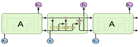
In a NN with a single hidden layer, the number of input layer nodes is always proportionate to the size of the data and the input layer nodes are synaptically linked to the hidden layer. The weight coefficient between each pair of nodes from (the input to the hidden layer) determines the node's importance and whether the information will be passed on to the next layer. While learning the latent weight update process, the artificial NN will learn the appropriate weights for each individual synapse after learning is finished. The input and bias amounts, along with each importance, are added up and multiplied. This information is then sent to the hidden layer nodes using the SoftMax function to a sigmoid or tangent hyperbolic (tanh) function, which is known as the activation function. The numbers produced by this transformation need to have the lowest feasible error in the train after training, which can be verified in the test set. The values acquired due to this modification make up the NN's output. In this case, to get the most out of the model, the output layer and hidden layer are connected using a back-propagation approach, and the back-propagation process will be finished by delivering a signal that conforms with the ideal weight and ideal error for the chosen number of epochs. This approach will be used again to improve our forecasts and reduce mistakes. After this stage is finished, the model will have been trained. Recurrent neural networks (RNN) are a family of NNs that anticipate future value based on a previous sequence of observations; this kind of NN uses earlier stages to learn data and forecast patterns. To estimate and forecast forthcoming values, it is necessary to remember the data past locations. In this instance, the hidden layer stores the previous data from the sequential sequence. The approach of predicting future data based on the characteristics of earlier lines is referred to as "recurrent" in this context. Because RNN cannot store long-term data, using Long Short-Term Memory (LSTM) based on a "memory line" has proven to be quite beneficial in correctly predicting future scenarios involving long-term sequential data. Prior-stage memory may be stored in an LSTM employing gates with an integrated memory line. The diagram below demonstrates the structure of LSTM nodes.
In contrast to other RNNs, LSTM is capable of recognizing data sequences and making predictions accordingly. The top line of each cell serves as a transport line, carrying data from the previous cell state to the present, and cell autonomy enables the model to filter or add values from the last cell to the current cell. Each LSTM node must comprise a collection of cells accountable for storing the sequence from the sequential data. The sigmoidal neural network layer, including the gates, optimizes the cell's value by deleting or permitting input to pass. A binary value (0 or 1) is assigned to each sigmoid layer, where 0 denotes "let nothing through" and one indicates "let everything through." To control the state of each cell, the gates are managed as follows:
The output of the forget gate is a value between 0 and 1, with 1 denoting "totally keep this" and 0 denoting "absolutely disregard this."
Which new data will be saved in the cell is determined by the memory gate. A sigmoid layer's initial "input door layer" determines the values to be modified. The next step is to create a vector of potential new candidate values that could be added to the state using a tanh layer.
The output gate determines the output of each cell. The cell state and the current filtered and added data will both affect the output result.
2.2. Related works
Much work has been done in HUIm; the most relevant results related to the proposed approach are discussed. When exploring the domain of e-commerce/ retail for HUIM, N. Guo et al. devised a technique for extracting high-utility item sets from online retail data; the authors suggested a brand-new approach dubbed HUIF (Lin, Zhang & Fournier-Viger, 2017). To narrow the search field and expedite the mining process, HUIF employs a heuristic methodology. A real-world dataset from an online retailer was used to evaluate the algorithm, and the findings revealed that HUIF outperformed existing algorithms in terms of mining time and memory use. This is explored in a distributed fashion by García-Sánchez et al. (2005) where online e-commerce data is presented as an incremental and distributed approach. The algorithm can manage both the considerable volume of transactions and the dynamic nature of the data. The authors evaluated the method on a sizable dataset from an online retailer, and the findings demonstrated that the system could manage the mining operation well. X. He and colleagues suggested utilizing Apache Spark to implement a parallel algorithm for mining high-utility item sets from massive e-commerce data (Gan, Lin, Zhang, Yin, et al., 2021). The algorithm can be deployed over numerous nodes for parallel processing and managing high volumes and velocities of data. The results of the algorithm's evaluation on a dataset collected from a Chinese e-commerce website demonstrated that the algorithm could manage the mining task successfully and efficiently. A parallel technique named PHUI-Miner was developed by Yin et al., (2021) to mine high-utility items in e-commerce datasets. This approach is on par with many innovative algorithms using several sizable e-commerce datasets. According to their findings, PHUI-Miner performed superiorly in execution speed and scalability. For mining utility itemset in e-commerce datasets, Li et al. suggested a hybrid technique dubbed UIMiner-H. The method is evaluated against several other algorithms using various real-world data mining sets to determine its efficacy. Their findings demonstrated that UIMiner-H performed better in terms of efficiency and efficacy (Lin, Zhang & Fournier-Viger, 2017).
Similarly, innovative approaches such as Apriori and genetic algorithms were also used. Zhang et al. (2019) used a genetic algorithm for mining high-utility item sets from e-commerce data (Gan et al., 2019). The algorithm improves the efficiency and efficacy of the mining process by combining the benefits of genetic algorithms with pattern growth algorithms. A dataset from a Chinese e-commerce platform was used to evaluate the algorithm, and the findings indicated that it could find high-utility item groups that are beneficial for business applications. (Dong et al., 2020) used weighted negative utility and correlation-based pruning; the authors proposed a novel technique for mining high-utility item sets from online transaction data (Lin, Zhang, Fournier-Viger et al., 2017). The system can manage the uneven distribution of the data and can exclude unfavorable candidate item sets using correlation-based metrics. The technique was evaluated on several real-world datasets by the authors, and the results revealed that it can find high utility item sets beneficial for business applications. (He et al., 2022) suggested a unique two-step technique for mining high utility itemset from online e-commerce datasets. The Apriori method was used in the first stage to mine frequent item sets, and a utility-based pruning strategy was used in the second step to discover utility item sets (Duong et al., 2020). (Ghadekar & Dombe, 2019; Pillai & Vyas, 2015) suggested that the unique HUIM-Miner method be used in another work to mine high-utility items from online e-commerce datasets. The suggested algorithm employed a hybrid strategy to find high-value itemset that coupled the Apriori algorithm with a utility-based pruning mechanism. In subsequent research, (Rahman et al., 2022). Sra and Chand, (2024) proposed an improved technique for mining high value itemset from online e-commerce datasets. The efficient depth-first search method utilized by the suggested algorithm, HUIM-EDR, decreased the search space and increased algorithm efficiency (Nam et al., 2020). Chen et al. used a practical HUI-Max approach for mining high utility itemset in transactional datasets. The approach can be compared against current state-of-the-art algorithms using a variety of real-world datasets, including e-commerce datasets. According to their findings, HUI-Max performed better than the other algorithms regarding memory use and execution time (Xiong et al., 2018) expanded this by introducing a unique HUI-Miner technique to find high-value itemset in e-commerce datasets. This approach employs a hybrid search strategy (Lin, Yang et al., 2016). The result shows reliable performance against several innovative algorithms using synthetic and real-world datasets. According to their findings, HUI-Miner performed better regarding memory usage and time taken for execution (Duong et al., 2018). A novel HUI-TS approach was introduced in a different work by Liu and Qu, (2012) for mining high-utility itemset in time-sensitive e-commerce datasets, making their model performance at par with several existing algorithms using various real-world datasets. According to their findings, HUI-TS performed better in efficiency and efficacy (Li et al., 2023). A brand-new plan named UIMiner was put out by Li et al. (2023) for mining utility item sets in e-commerce datasets. The evaluation of the algorithm was compared against a variety of real-world datasets and with a variety of innovative algorithms. Their results indicated that UIMiner outperformed other systems in terms of efficiency and efficacy. UIM-Span is a practical approach that (Shankar et al., 2009) suggested for mining utility item sets in e-commerce datasets. Using several real-world datasets, they assessed their method and contrasted it with several other algorithms (Song et al., 2014). Their findings demonstrated that UIM-Span performed better than the other algorithms in terms of execution speed and memory use. An approach named UIMiner-T was put out by Liu and Qu (2012) in different research for mining utility item sets from time-sensitive e-commerce datasets. The algorithm was tested on several real-world datasets and contrasted it with other innovative algorithms. Their findings demonstrated that UIMiner-T performed better in terms of efficiency and efficacy (Li et al., 2023) For mining utility itemset in e-commerce datasets with limitations (Wu et al., 2021) suggested a unique technique dubbed UIMiner-C. Using several real-world datasets, they assessed their method and contrasted it with several other algorithms. According to their findings, UIMiner-C fared better than the different algorithms in terms of efficacy and efficiency.
Overall, the literature suggests several efficient and effective algorithms are available for mining utility itemset in e-commerce datasets. Researchers have proposed various techniques, including time-sensitive and constraint-based mining, to manage the dynamic nature, high velocity, and volume of online transaction data and hybrid mining to improve the efficiency and effectiveness of these algorithms. The algorithms can be parallelized and distributed over multiple nodes for efficient processing and can manage the imbalanced nature of the data using negative utility and correlation-based measures. Further research is needed to develop more efficient and effective algorithms to address the increasing volume and velocity of online e-commerce data (Sohrabi, 2020).
The main problem is that high utility itemset mining aims to find the items that make more profit. This concept applies where yields are based on individual articles, which offers enormous profits. The main issue with this approach is that it is still being determined when the item will be sold. To overcome this issue, a model is developed to predict what will be sold. This will solve two problems. The first is inventory management, as the items predicted by the proposed model will be sold. The second is identifying similar groups of people. This will ensure a more appropriate categorization of the customers coming. This approach to finding high-utility items based on upcoming events is new and has yet to be explored (Song et al., 2014). Sukanya and Thangaiah (2023) proposed a HUI mining algorithm technique based on differential evolution and particle swarm optimization on voluminous transactional databases. Loukili et al. (2023) have successfully created an algorithm that utilizes association rules and the Frequent Pattern-Growth algorithm to provide personalized recommendations to consumers. and yielded favorable outcomes, including a high average probability of purchasing the subsequent product recommended by the recommendation system. Xue et al. (2017) propose a novel matrix factorization model with neural network architecture by creating user-item matrix for item prediction. Umayaparvathi and Iyakutti (2017) proposed a CNN-based solution by identifying customer attributes. Premanand G. et al proposed a CNN-based technique that uses the product history of the customer and the linkage between the same products bought by other customers to find high-utility products. Pazhaniraja et al. (2021) have used the random forest to predict the next order in an online grocery store depending on the transactions. Siva and Chaudhari (2024) has proposed a convolutional sequential semantic embedding technique for predicting top n recommendations and high utility itemset over sequential transactions.
3. Methodology
3.1. Proposed approach
In Figure 2 this study aims to construct and develop a deep learning-based system for anticipating and examining online grocery orders. A Long Short-Term Memory (LSTM) focuses on feature extraction and pattern detection in the analysis to predict how many groceries will be needed in the inventory. This saves time and effort and lets you find the most popular products, helpful items, etc. Time series is an integral part of statistics and machine learning that is often overlooked in data mining. This way of predicting grocery sales will help companies meet customer demand for goods and group customers with similar tastes. This will also boost client happiness and create opportunities (Pillai & Vyas, 2015). Although time series analysis and forecasting have been well studied, only some research publications apply LSTM to real-time, live data in this domain. By pulling out time series patterns like seasonality or trends, grocery stores will better manage their logistics. An architecture was created using internal data that collects customer details and the items they bought from the shop over time to offer the best solution. The architecture does data preprocessing, which also finds their features and patterns (Gan, Lin, Zhang, Fournier-Viger, et al., 2021). Finally, an LSTM was created to solve the problem of anticipating the grocery requirements for the specified period using all the information learned during the analysis step. The proposed approach compares the data produced by the model with the actual demand for the products to validate the architecture and the deep learning-based artificial intelligence model.
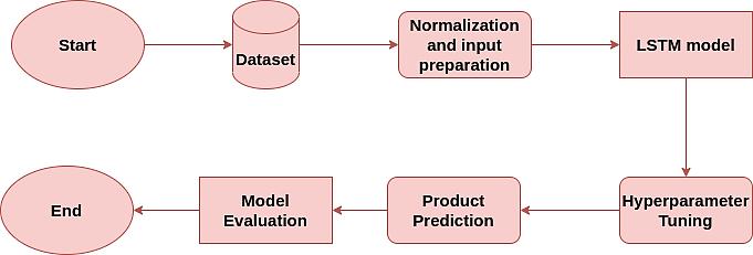
The proposed approach has used Instacart, a grocery ordering and delivery app, as the dataset to develop the proposed model. There are over 300 million transaction data from more than 200,000 Instacart users. Here, it helps to identify all the patterns and habits of what consumers buy and what they will need in the future. The proposed model predicts which previously purchased products will be in need in future orders and keeps track of items needed if a previous customer comes again, which is done by finding the reorder pattern of the existing customer. Once the model is trained, it can identify future needs.
The input sequence in itemset mining uses the short-term memory from the preceding cell and the long-term memory from the previous cell state at a particular time t. Thus, LSTM will use two types of information to make it accurate. The forget gate will find and only keep the relevancy of the information passed from the earlier cell state after the sigmoid layer converts the translated information from the current input and the previous cell into a value between 0 and 1. Non-important pieces of information are then deleted. When the value is 1, all data is saved in the cell; however, when the value is 0, all data from the earlier state is erased. Like the output gate, the input gate specifies which data the change gate should update. Which data from the present cell state should be the output gate determines output (Fournier-Viger et al., 2019).
The aim of developing this model is to predict the grocery requirement in the future from the analysis of current and past orders. To achieve this, LSTM architecture is proposed, which takes input from the existing orders and predicts future orders, as it is evident that around 60% of the items are reordered. This prediction of future grocery items will help to maintain the required stock (Luna et al., 2023). By predicting future orders, it is evident that the high-utility item can be restocked.
The data needed to predict future demands which are finding the user (use_id), the product's the user buys (product_id), the day in the week when the order is placed, the hour of the day when the order was placed, and the time since the last order, which is used to predict the product_id to be purchased in the upcoming days. With the use of a multivariate sequence of input variables and supplied multivariate grocery time series data collected from multiple sources, the suggested model aims to anticipate future demand (Liu et al., 2005). The following LSTM implementation strategies are being assessed to fulfil this assignment from the original dataset modified. Moreover, a continuous sequence is used to build an input sequence that includes the crucial dimension of the LSTM design. Figure 1 depicts the recommended model framework.
The input sequence consists of k = 5 (user (user_id), the product's user buys (product_id), the day in the week when the order is placed, the hour of the day when the order was placed, the time since the last order) features with a time step of m, as seen in the above section of the image. The LSTM is supplied with the input Xt1 at time t1, a 5 m matrix correlated with ht2 and ct2. The second stage's LSTM takes as inputs the output ht1 of the earlier stage, the input sequence Xt, and the cell memory ct1. This procedure is conducted four times until the final input sequence Xf and corresponding output hf, a vector of length equal to the number of neurons in the final LSTM layer, is obtained. hf is finally sent to a fully linked layer, as seen in the last part of Figure 3, where a linear activation function is used to estimate the closing products. The output will be a multilabel classification where every item in the inventory for the future is predicted. If the label output is 1, then the item will be needed in future order, and if the output is 0, the item is not needed in future order for the current time step. The average frequency of each item that is regularly purchased by the customer is fixed as the quantity of that item. For example, we can have only 5 items in our itemset that are: Milk, oil, banana, strawberry, and tea. So, if our predicted output is 01100, this means only oil and bananas are purchased in the next order. The quantity is the average amount of the items the customer buys, which is 1ltr for oil and 6 bananas (Lin, Yang et al., 2017).
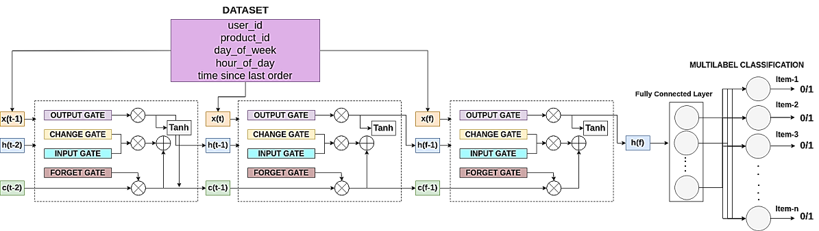
Figure 3 The proposed model architecture for product prediction using LSTM and multilabel classification.
The architecture of the LSTM is a 4-layered LSTM stacked upon each other; a linear layer follows this. The input to the network is the data discussed above. Then, for each time stamp, the hidden and cell states are found for each layer, and the last hidden state is given to the linear layer, which predicts the product_id, which will be purchased in the future. While training, 10,000 future items are expected, and the loss is calculated and backpropagated by comparing all the future predictions. The proposed approach will use an LBFGS (Limited-Memory Broyden-Fletcher-Goldfarb-Shanno) optimizer to train the model and an MSE (Mean squared error) loss to measure the accuracy of our model. At the same time, training the model, the future prediction made by the model, and the failure to finetune the model (Nam et al., 2020). The training was done on an Rtx-5000 GPU, and it took around 32 hours to converge and give a reasonable accuracy. After successful movement, the model predicts up to 10,000 future orders successfully.
The architecture of the LSTM is a 4-layered LSTM stacked upon each other. This is followed by a linear layer. The input to the network is the data discussed above. Then, for each time stamp, the hidden and cell state is found for each layer, and the last hidden state is given to the linear layer, which predicts the product_id that will be purchased in the future. While training, 10,000 future items are predicted, and the loss is calculated and backpropagated by comparing all the future predictions((PDF) a predictive analytics model for maximizing profit in e-commerce companies, n.d.). The proposed approach will be used using LBFGS (Limited-Memory Broyden-Fletcher-Goldfarb-Shanno) optimizer to train the model and use MSE (Mean squared error) loss to measure the accuracy of our model. While training the model, the future prediction is made by the model and the loss to finetune the model (Lai et al., 2023). The training was done on an Rtx-5000 GPU, and it took around 32 hours to converge and achieve good accuracy. After successful training, the model predicts up to 10,000 future orders successfully (Nam et al., 2020).
When the input is embedded in the hidden space, every recently purchased item can be clubbed together. Similarly, the cell state will contain more frequent item embedding but for long sequences. Hence, the combination of recent and the whole sequence finds every type of small and large product pattern, making the model perfectly accurate for future prediction. The model also considers the recurring customers and caters for their needs. Implementing this strategy to estimate the item adds extra dimension, such that there can be a reduction in item sets by discarding items that are impossible to be of high utility or not involved in the search space.
3.2. Data description
The Instacart data from the app is the dataset that is analyzed. This data consists of a relational set of transactional data that tracks the orders of clients over time. To determine HUI, the goal is to predict which items will be in a user's future order (high utility Itemset). Around 200,000 Instacart members contributed over 3 million food orders to the dataset, which is anonymous. Values between 4 and 100 of each user's orders and a list of the things they bought when.
The description of the dataset is as follows:
Aisles: There are 134 distinct aisles in this file, each of which is different.
Departments: A total of 21 distinct departments are represented in this file.
Orders: This file includes all the orders that various users have placed. The following may be inferred from the analysis below:
206209 users have placed 3421083 orders.
The three sets are the prior, train, and test sets of orders. While order distributions in the train and test sets are comparable, order distributions in the prior set are different.
The range of a customer's total orders is 0 to 100.
Based on the plot of "orders vs day of week," thus map 0 and 1 as Saturday and Sunday, respectively, on the assumption that most people buy food on the weekends.
Most orders are placed during the day.
The 7, 14, 21 and 30 peaks in the "orders vs days since prior order" graph indicate that customers only place one order weekly.
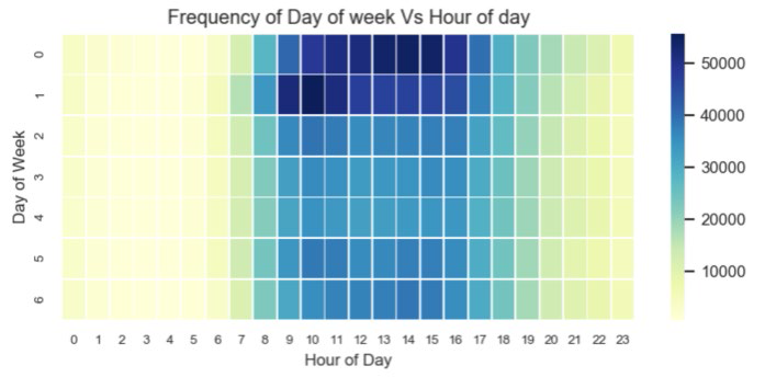
Based on the relationship between "day of week" and "hour of day," it is inferred that Saturday afternoons and Sunday mornings are the busiest periods for orders.
Products: This file includes a list of all 49688 items, together with information about each one's aisle and department. Different aisles and sections have varying numbers of merchandise.
Order_products_prior: This file contains details on the products that were ordered and the order in which they were put in the shopping cart. It also discloses whether the goods were reordered.
Order_products_train: This file contains details on the items that were ordered and the order in which they were put in the shopping cart. It also discloses whether the goods were reordered.
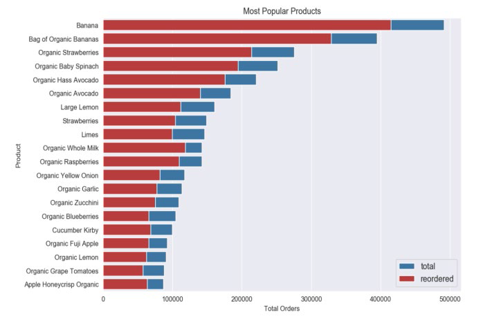
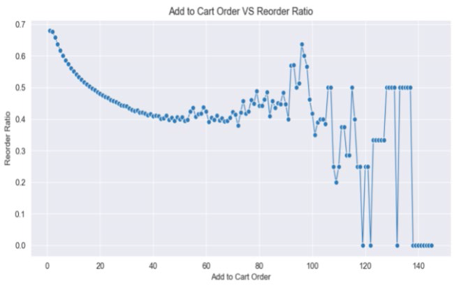
Here is some visualization in Figure 4, 5 and 6 on the dataset, which can be seen here: The hour from 9 to 5 is busy, and that is the time when a customer orders the most. The list of most popular items here can also be seen, which changes over time depending on the demand. Here is the pattern of re-ordering pattern of existing customers.
4. Results
4.1. Data preprocessing
Data preprocessing is a crucial step in our analysis, where raw data is cleaned, transformed, and organized to prepare it for further analysis. The first step is identifying missing values in the dataset and replacing missing values with estimated ones. Then we dealt with outliers and standardizing formats. This is followed by normalization or scaling of data to ensure that all features have a similar scale. It may also involve encoding categorical variables into a numerical format. At last, normalization is performed by scaling numeric data to a standard range, often between 0 and 1, to prevent certain features from dominating others. and transforming continuous data into categorical data. The dataset is also reorganized and split into train and test sets. The objective is to precisely predict the product that will be bought in the future and exhibit complex, distracting, and volatile behavior.
4.2. Model performance metrics
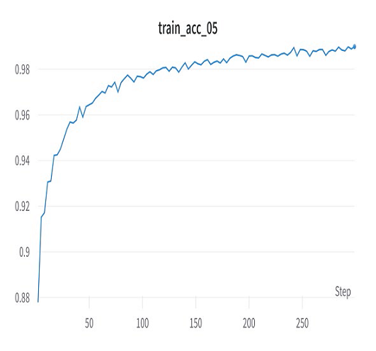
The model's accuracy is around 98%, even though the repeated orders are about 60 %. Still, accuracy was high due to finding large and small patterns, which not only see the products that consumers purchase every time but also keep track of the products purchased occasionally. This gives the original advantage of LSTM over other regular mining models, which is proven by the accuracy of predicting 10,000 items in advance. The accuracy was calculated by finding the several types of products ordered, the quantity of each product, the user who requested the product, and the amount of the product called by each user. The model is trained for 250 epochs. We have used the Adam optimizer with a learning rate of 0.0001. We have employed early stopping so that the model does not overfit.
A four-layered LSTM architecture is used to anticipate the product. Several options with varying numbers of neurons are considered within each of these models. These models' prediction accuracy and dependability are evaluated using three separate performance metrics: RMSE, MAPE, and R. These measures are defined in their analytical form as follows:
Where,
𝑦𝑖: Original sequential data,
𝑦𝑖: The average value in the original sequential data,
𝑦𝑖: Predicted sequential data calculated by the model,
𝑦𝑖: Average value of the predicted sequential data,
𝑁: Number of observations.
The corresponding precision between the absolute and predicted values is calculated by the relative average of the error (or MAPE) metric, the fundamental and predicted values are determined by the R metric and the square root of the mean square error of the actual and estimated values is measured by the RMSE metric. When the RMSE and MAPE values are lower, the model has achieved good accuracy and precision. On the other hand, a higher R-value suggests that the expected and actual sequences are comparable. The model's forecast for a particular phase was not directly compared to the actual output; instead, the number of different product types and the quantity of each product were measured, and this information was utilized to determine all the matrices. Suppose it is tried to compare each transaction. In that case, the error will be high. Also, it needs to make sense to give the correct criteria as the focus is on finding various products that consumers will require, and the order of finding the products is not an important feature. Also, the predictions calculated using the normalized data are transformed in the opposite direction to provide performance metrics. The model is independently run several times to address and eliminate stochastic behavior. The typical MAPE and R scores are displayed in Table 1. The proposed approach used four different models and found that the four-layer LSTM-based model was optimal.
Table 1 RMSE, MAPE, and R values for predicting 10,000 items to be purchased.
| 3
Layer LSTM |
5
Layer LSTM |
7
Layer LSTM |
4
Layer LSTM |
||
| RMSE | MIN | 34.73 | 43.82 | 38.55 | 37.27 |
| AVERAGE | 49.95 | 57.07 | 47.19 | 42.7 | |
| MAX | 77.48 | 72.16 | 60.74 | 49.49 | |
| STD | 9.77 | 8.08 | 4.96 | 2.95 | |
| MAPE | MIN | 0.75 | 0.89 | 0.76 | 0.72 |
| AVERAGE | 1.12 | 1.23 | 0.97 | 0.86 | |
| MAX | 1.61 | 1.5 | 1.24 | 1.1 | |
| STD | 0.25 | 0.17 | 0.099 | 0.0912 | |
| R | MIN | 0.99 | 0.99 | 0.99 | 0.99 |
| AVERAGE | 0.99 | 0.99 | 0.99 | 0.99 | |
| MAX | 0.99 | 0.99 | 0.99 | 0.99 | |
| STD | 0.0006 | 0.0007 | 0.0003 | 0.0002 | |
The primary model selection criteria are the average RMSE score produced from these several repetitions. A model with the lowest RMSE, MAPE, and highest R values are considered good.
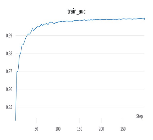
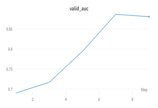
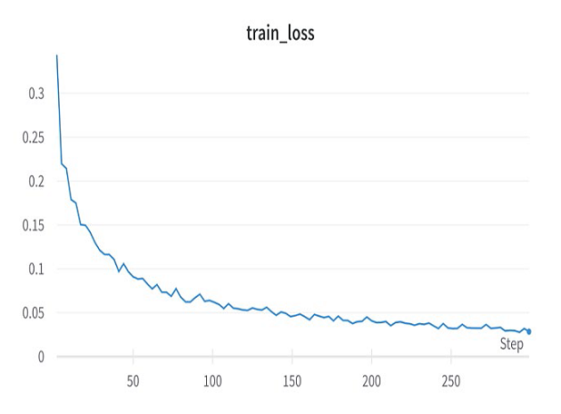
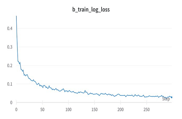
The graph Figure 7, 8, 9, 10 and 11 for training AUC (Area Under Curve) is given, which clearly shows the model correctly predicts future orders. Thus, AUC is almost one for training and 0.9 for validation. The value of loss and log loss while training is 0.05, boosting the accuracy to 98%.
4.3. Discussion
The main aim of this approach is to provide inventory management to maximize profit. The higher accuracy of the model suggests that the item that will be required in the future is correctly predicted using LSTM. This includes both the items that are demanded in huge quantity and have less profit per item as well as less demanded items that have higher profit per item. This is achieved using LSTM as the global objective is to maximize the profit and due to the architecture of LSTM, both cases are covered. Once the LSTM is trained, we have evaluated our model and have an accuracy of 98%. We used RMSE, MAPE, and R values to validate the accuracy and fix the best architecture suitable to us. To calculate the loss between the predicted and absolute value, RMSE uses a simple distance between the items in the 2-D plane while MAPE measure the distance in the 1-D plane and the R score identifies the relation between dependent and independent items purchased. This way, our approach not only finds the best architecture for prediction but also uses different metrics so that the predicted and absolute items chosen are the same, as well the sequence of choosing the items can be closer. The focus is also given to the item, often taken in pairs, so the prediction can be as accurate as possible.
4.4. Relationship between effectiveness vs. average transaction size of customer
Various customers have different tractions, which include other items. Traditional item-set mining considers individual items. Still, our model focuses on multiple things simultaneously, maximizing the total profit by keeping everything in the inventory beforehand. Another observation is that the number of transaction-weighted utilizations of any itemset X is defined as the sum of the transaction utilities of all the transactions containing X. This overestimation worsens as transactions become more extended because more significant transactions tend to involve more unrelated things. Despite the overestimation, Phase I's efficiency is clear. As a result, our suggested approach performs better, especially in dense databases.
4.5. Comparison with existing techniques
In this section, we have compared our approach with some existing approaches that use machine learning and deep learning for the prediction of high utility itemset. It can be seen in Table 2 and the accuracy of our approach outperforms the existing techniques.
5. Conclusion
The region of most excellent attention is itemset mining, which is what will come next. However, accurate and consistent product prediction is challenging because of its chaotic and nonlinear behavior. Market data, macroeconomic data, and other factors impact output predictions. This study focuses on building LSTM-based models to anticipate the product that will be in demand in the future so that customers can get the things they desire, merchants can know what to provide, logistics management is simplified, and profit is increased. The LSTM model was implemented, and its performance was assessed using various assessment criteria to verify the model. A four-layer LSTM model may offer the best fit and excellent accuracy for prediction, as per the experimental data. The suggested method can be used in other key market segments where the data indicates an equivalent tendency. The development of predictive model’s hybrid using the LSTM or other sequence models, making more sophisticated neural networks. This can be used with existing data mining architectures and is another intriguing field for future study. In addition, the proposed method trains the model parameters using hybrid optimization methodologies such as genetic and particle swarm optimization algorithms to improve prediction accuracy even more. The only shortcoming of this approach is that the addition of the latest items in the inventory requires retraining of the model.

