


 nueva página del texto (beta)
 Inglés (pdf)
 Artículo en XML
 Referencias del artículo
 Enviar artículo por email
 Citado por SciELO
  Similares en
SciELO
Similares en
SciELO 
 Permalink
1. Introduction
Using fundus images to diagnose ocular pathology is quite challenging in the medical field (Elloumi et al., 2019). Any disorder or condition impairing the eyes' capability of functioning properly or negatively affects their visual acuity is referred to as ocular disease. Almost everyone goes through visual problems at some point in their lives. A few are teenagers who can receive treatment at home or don't show up on claims, whereas others require a specialist's help (Khan et al., 2022). Fundus issues are the most common cause of blindness worldwide. The most prevalent eye conditions are age-related macular degeneration (AMD), cataracts, diabetic retinopathy (DR), and glaucoma. According to pertinent studies, by the year 2030, there will be more than 400 million individual suffering from DR (Adio et al., 2011).
Those ocular conditions are currently one of the major global healthcare problems. The most important concern is that the ophthalmic condition is potentially fatal, resulting in permanent blindness for individuals. Early diagnosis of various conditions in medical settings helps stop eyesight problems. Thus, it is essential to discover eye issues using automated computer-aided diagnostic methods (Adio et al., 2011). Automatic sickness diagnosis is one of the most crucial milestones in reducing ophthalmologist's workload. Electronic support is always needed by medical facilities for helping them detect specific disorders more accurately. Tasks that could considerably benefit from computerization, such as large-scale data collection, data structure and classification, complex input analysis, relationship identification, and others, may benefit from this assistance. Without involving humans, diseases can be identified with the use of DL and computer vision techniques. Even though much research have yielded positive results, only few have been able to accurately identify a variety of eye illnesses. More investigation is required to completely comprehend the many features of fundus imaging for efficiently diagnosing a broad spectrum of ocular conditions.
This study offers a DL-based method to classify different eye conditions. The research paper's remaining sections are organized as follows: first, a brief description of the database that has been used. After that, the steps for the pre-processing and feature extraction have been explained. Following a discussion of the findings in part four and an explanation of DL methods used for predicting eye disorders in section three, the research is concluded.
2. Related work
Badah et al. (2023) carried out autonomous detection of eye diseases using machine learning (ML) and deep learning (DL). A total of six ML techniques is used by the classification systems: Support Vector Machines (SVMs), K-nearest neighbors (KNN), Naïve Bayes (NB), multilayer perceptron (MLP), decision tree (DT), and random forest (RF). DL models, like the convolutional neural networks (CNNs) depending upon the Resnet-152 model, is the second option. The proposed approach was evaluated using (ODIR) dataset. In the case when compared to other ML classifiers, the collected data revealed that RF and MLP classifiers had the highest level of accuracy, at 77%. For the same dataset and task, DL model (CNN model: Resnet152) offers a level of accuracy of 84%, which is significantly greater compared to the prior model.
Khan et al. (2022), suggest using DL for ocular diseases recognition. ODIR dataset that comprises 5000 images of eight different types of fundus has been classified with the use of state-of-art image classification algorithms like VGG19. For these classes, the dataset is incredibly uneven. In order to solve this type of challenge, the study suggested taking the same number of images and converting multi-class classification problem to the binary classification problem. Then VGG19 was used to learn the binary classifications. In normal (N) vs. pathological myopia (M) class, 90.94% vs. glaucoma (G) class, and 94.03% vs. cataract (C) classes, this model had an accuracy of 98.13%. The accuracy of the other models rises as well in a case where the data is balanced.
Prasad et al. (2019) created a model with the use of DNN, multiple eye diseases can be found. The proposed DNN model is useful in glaucoma and diabetic retinopathy early detection. It can make patients want to visit an ophthalmologist for a screening. The developed model was less complex and generated 80% accuracy.
Guergueb and Akhloufi (2021) have described an approach for detecting ocular diseases with the use of recent DL methods that has undergone a number of refinements. With AUC of 96.04% for 8 diseases and AUC of 98.31% for 6 diseases, results demonstrate that the best model performs well.
Gour and Khanna (2021) employ multi-label, multi-class ophthalmological illness diagnosis using transfer learning (TL)-based CNN. The proposed method leverages ODIR database for finetuning 4 state-of-art pre-trained CNN architectures. Based upon parametric evaluation of training, validation, and testing phases, VGG16 network outperforms CNN designs of Inception V3, MobileNet and ResNet. F1 score and AUC of the VGG16 two input approach with SGD optimizer have been 85.57 and 84.93, respectively. In comparison to other architecture, the concatenated input method with the VGG-16 architecture, represented as Model2, had also shown increased F1 and AUC score with VGG16 applying SGD optimizer, i.e., 85.57 and 68.88.
Li et al. (2022) created a multi-label classification regarding fundus disease using binocular fundus images as well as an NN algorithm model that relies upon attention mechanisms and feature fusion. Through tests on test images, this technique achieved the following values: 94.23%, 99.09%, 99.16%, and 99.23% for accuracy, precision, F1, and recall.
Shamsan et al. (2023) suggest automatic fundus color image classification for prediction of types of eye disease. Three classification algorithms for CFP images were developed depending on hybrid features to diagnose eye diseases. First, an ANN with the features from the DenseNet-121 and MobileNet models independently is utilized for classifying an eye illness dataset. This is done after the principal component analysis (PCA) has been applied to eliminate repetitive features and the high dimensionality. The second approach involves employing an ANN for classifying the dataset for eye diseases with the use of features that were fused from the DenseNet121 and MobileNet models both prior to and following feature reduction. The third approach combines hand-crafted characteristics from the DenseNet121 and MobileNet models with ANN for classifying the dataset for eye diseases. ANN achieved an accuracy of 98.5%, an AUC of 99.23%, a specificity of 99.4%, a precision of 98.45%, and a sensitivity of 98.75% depending on the combined MobileNet and handcrafted characteristics.
ML algorithms, including RF, DT, NN, and NB algorithms, were applied to analyze patient data according to various attributes, including clinical observations, age, and history of illness (Malik et al., 2019). The authors have introduced their data driven method for eye disease classification with ML. Due to the structured data organization, the DT and RF algorithms have a prediction rate of no less than 90%, which is higher than that of more complex methods like the NB algorithm and NNs.
In this study, we presented an advanced model for diagnosing eye diseases using fundus images, which represents a significant contribution to the field of medical imaging and ophthalmology. Following is a detailed description of our contributions:
- Novelty: Our model leverages deep learning techniques, specifically convolutional neural networks (CNNs), to classify different types of fundus images into distinct classes representing different visual disorders. The use of the ODIR dataset, which includes 5000 images covering eight fundus types, is characterized by the breadth and diversity of eye conditions. This approach demonstrates the effectiveness of CNNs in processing and analyzing complex medical images and is an innovative advance in this field.
- Importance: The performance metrics achieved by our model are exceptional, with recall, precision, and F1 scores reaching 99.9%. This level of accuracy is critical in medical diagnosis, as accurate disease classification can significantly impact patient outcomes and treatment strategies. The integration of TensorFlow as a back-end framework enhances the model's efficiency and scalability, making it a valuable tool for medical practitioners in real-world environments.
- Scope: The model is designed to handle a range of sample disturbances, as represented in the dataset. The ability to classify these disorders with high accuracy underscores the strength of the model. However, the study acknowledges limitations related to small sample sizes for some rare diseases, which may impact classification performance. Future research aims to address these limitations by incorporating more diverse and comprehensive datasets.
- Integration: Our findings contribute to existing research by demonstrating how deep learning models can be effectively applied in diagnosing eye diseases. This model not only matches existing methods in terms of accuracy, but surpasses them, providing a potential paradigm shift in how ocular disorders are identified and classified. The study suggests that with further improvement and additional data, the model could become more valuable for clinical applications, especially in diagnosing rare eye conditions.
In summary, our work provides a significant enhancement to the field of eye disease diagnostics by applying cutting-edge deep learning techniques. It provides a promising direction for future research and has the potential to improve diagnostic accuracy and clinical practice in ophthalmology.
3. Methodology used
3.1. Model diagram
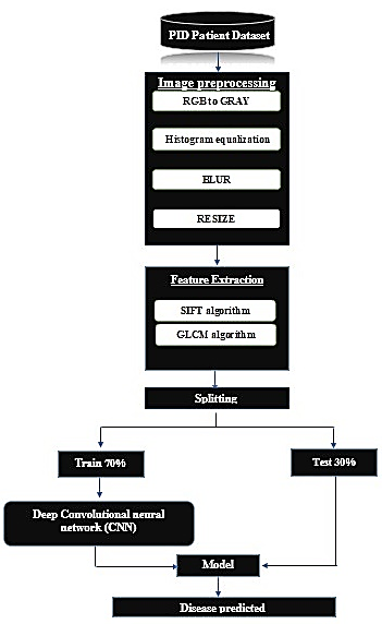
Figure 1 depicts a model schematic of the recommended procedure (flow chart of the deep conventional neural network classifier).
3.2. Dataset used
We used a well-known platform in the field of machine data analysis, which provides a wide range of databases in various fields, including medicine and diseases. We used a database from Kaggle related to eye diseases which helped us in analyzing the data and developing the models.
In the field of ophthalmology, early fundus screening is a cost-efficient and successful method that is used to prevent eye diseases-related blindness. Clinically, manual diagnosis takes a long time and can cause the problem to worsen because of a lack of medical resources. Certain studies on ocular diseases have shown promising outcomes with the advent of DL; nevertheless, most of these studies focus just on a single condition. In fundus screening, ophthalmologists typically detect multiple diseases based on binocular fundus images. For better reflecting real medical environment, we have released a dataset comprising eight disorders.
The dataset utilized in the presented work is called ODIR (ocular disease intelligent recognition). One of the most complete datasets to diagnose eye illnesses that is publicly accessible on Kaggle is ODIR. This dataset's fundus images are classified into eight groups based on eye diseases. A total of seven disease classes are included in such categories, that is, Hypertension (H), age-related macular degeneration (A), myopia (M), normal (N), Glaucoma (G), cataract (C), diabetes (D), other diseases/abnormalities (O).
3.3. Digital image preprocessing
The acquisition of images has increased in numerous applications, making image preprocessing an important area of research. Prior to applying any additional methods to the image, a series of activities known as "digital image preprocessing" should be carried out on the image which was entered into the Diagnose system to enhance it. The necessity of preprocessing is important since it will help in the later stages of Diagnose system by eliminating any unnecessary data (Plataniotis & Venetsanopoulos, 2000).
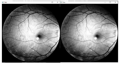
Preprocessing procedures (Figure 2): 1) RGB image conversion to grey scale, 2) histogram equalization, 3) blurring, 4) resize image.
3.4. Preprocessing procedures
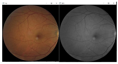
Convert the image to grayscale color format: 1) the inputted image changes color at introduced time, switching from the imitation RGB color space to grayscale color space. This conversion occurs because an image in the grayscale color format just requires one channel to be saved and displayed on a computer, whereas an image in RGB (red, green, and blue) color space requires 3 channels. The goal of this type of conversion is representing an image with less data. By converting the colored images to grayscale, the processing performance is increased. Naturally, the intensity of such grayscale image is stored as an eight-bit integer number, offering 256 different possibilities for grey spectra, ranging from white to black. At this point in image preprocessing, every pixel in the inputted eye image-which has 24 bits-is converted to a grayscale color pixel with merely eight bits, 2) the next equation was used for image conversion from RGB to gray mode (Bala & Braun, 2003):
Figure 3 shows the converted image to gray level.
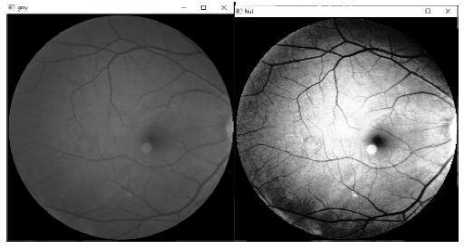
Histogram equalization (HE): It has been shown that HE method is a highly accurate way for combining colour and brightness data from significant local features in the color images. It also does an excellent job of reducing noise, blurriness, and contrast (Iwasokun & Akinyokun, 2014). To boost contrast in an image, the HE approach was applied. Mapping gray levels with input grey level probability distribution as guide is the basic notion behind it. Overall contrast is improved by flattening and expanding the dynamic range of image histogram (Sharma et al., 2012). This approach works best with images that have a dark or bright foreground and background, also basic foreground and background intensity (Elfarra & Abuhaiba, 2012). The following equation shows how to use the histogram cumulative distribution function for computing HE.
In which X denotes gray value and h represents image histogram.
Where, cdf(x)min: represents the minimum cumulative distribution function value, E*F: Columns and rows number of images, L: Grey level values utilized =256.
Figure 4 shows the result of HE of the gray image.
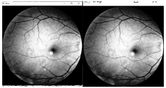
Blurring: blurring is accomplished through convoluting the image with low-pass filter kernel. Noise reduction benefits from image smoothing to remove noise or texture in small details. It is usually beneficial to apply image processing techniques that highlight the finer elements in the image (Zhang et al., 2012). There are several ways to perform such procedure. Typical filter types used in such methods include of: Gaussian filter, median filter, and mean filter. In this study, utilizing the Gaussian filter (5x5). Figure 5 shows the result of blurring.
Resize image: After resizing, the eye image is shown in Figure 6. In the presented study, all images have been reshaped with the use of (200*200) distances utilizing Bicubic Interpolation (Triwijoyo & Adil, 2021).
3.5. Feature extraction
One way for conceptualizing feature extraction could be as a particular dimensionality reduction type which was applied to image processing and pattern recognition. Finding the most important information in original data as well as displaying it in a lower dimensional space are the key feature extraction goals (Najah, 2017).
When input data is too large to analyze and is considered redundant (i.e., a lot of data, yet not enough information), this data will be translated into smaller set of features (which are referred to as features vector). Feature extraction represents the process of transforming input data to a feature set. In a case when the extracted features are carefully selected, the aim is that the feature set would use this reduced input representation instead of the full-size input before extracting the data from the input required to complete the intended task (Seeger & Laboureux, 2023).
Scale-invariant feature transform (SIFT) features extraction: To solve the issue of invariance to the rotation and scaling in feature extraction, SIFT approach was created (Lowe, 1999; Lowe, 2004). SIFT descriptors are relatively insensitive to changes in translation, illumination, rotation, and scaling. They also show certain invariance against affine distortion. Among the various computer vision applications which could benefit from the SIFT features is image classification. A comparison is made between features extracted from the image to be analyzed and those kept in a database of objects that have been identified. Furthermore, SIFT characteristics can be used for localisation, tracking, scene modeling, recognition, and 3D mapping (Wang et al., 2013; Yang et al., 2017; Bejinariu & Luca, 2018; Bejinariu et al., 2018).
There are four feature detection steps in SIFT:
1. Scale-space extrema detection: In spite of orientation or scale, a DoG function is utilized in the first stage for scanning all image locations as well as scales in search of possible interest points.
2. Keypoint localization: Low contrast areas and edges are eliminated from first stage locations using two different types of thresholds.
3. Orientation assignment: each one of the key points has at least one orientation assigned to it based upon local image gradient directions. Transformations are invariant because all subsequent operations have been carried out on the image data which had been modified to specified orientation, scale, and location for every feature.
4. Key-point descriptor: A description of local features around each keypoint was computed. Every feature descriptor can be defined as a vector of 128 dimensions which uniquely pinpoints the area surrounding the key-point. The descriptor depends on a local image gradient which has been rotated according to the key-point orientation in order to guarantee orientation invariance.
Since SIFT-generated attributes are frequently present in real-world images, a few of such descriptors should be used.
Gray level co-occurrence matrix (GLCM) Feature extraction: It is well known that through utilizing statistical intensity combination distributions at several points surrounding each other, 2nd-order statistical texture features could be recovered from images (Wang et al., 2013; Yang et al., 2017). There are three alternative orders in which statistics might be displayed, depending on the quantity of intensity points in an image. Although higher-order statistics are feasible in theory, their practical application is precluded due to their enormous processing costs. Texture features are used to describe the interaction and structure of surfaces in relation to their environment (Bejinariu & Luca, 2018). The inverse difference moment (IDM), entropy, correlation, homogeneity, sum variance, autocorrelation, contrast, dissimilarity, energy, IDM normalized, and maximum probability are 22 texture-based variables that were gathered. Some of them are expressed as follows:
Energy: Other terms for energy are uniformity and angular second moment. It gives the square element summation of the GLCM matrix. It functions by passing from homogeneous to non-homogeneous regions. It is higher when there are a lot of repeated image pixels.
Entropy: Image randomness is determined by it. Consequently, an image that is homogeneous will have lower entropy values.
Contrast: It measures the amount of contrast between a pixel and the pixels around it in the entire image.
Correlation: It is a measurement of linear gray tone dependency of the image. It explains how a pixel and its neighboring pixel are correlated.
Homogeneity: It describes the degree of pixel similarity. An image's homogeneous GLCM matrix indicates that its value equals 1. It is quite low in the case when the image texture simply requires minor modifications.
Where, Pij= (i,j) normalized GLCM matrix element. µ represents average GLCM matrix that has been assessed with the use of:
σ= denotes the intensity variance regarding all the pixels that were assessed with the use of:
N represents the number of the grey levels in the image.
3.6. Classification phase based on CNNs
CNNs represent significant types of the NNs utilized for image recognition. An image has been utilized as the input, and following the processing, it is categorized. For implementing CNN model, keras which is an open-source and free DL package, has been implemented. For the identification of an object that has a probability in the range of 0 to 1, every input image will be sent via a convolution layer succession that contains the filters (i.e., kernels), fully connected layers (FC), and pooling. Whether they have 1, 2, or 3 dimensions, CNNs operate similarly. What is different is the way the filter, which is also referred to as the convolutional kernel or a feature detector, traverses data and structure of input data. The current studies achieved 1D CNN layers' parameters will be discussed and illustrated in the following way:
1D convolution layer: A modified 2D-CNNs’ version that is called 1D-CNNs had recently been developed. Since 1D-CNNs just perform 1-D convolutions, they have an advantage of having low computational need, enabling real-time and affordable implementations of hardware. A convolution kernel produced through 1D convolution layer is passed through in order to produce a tensor of outputs in one temporal (spatial) dimension.
Max-Pooling: A new layer known as a pooling layer is added following the convolutional layer. After the convolutional layer's feature maps have been subjected to a nonlinearity (like ReLU). Maximum output might be achieved using Max-Pooling method. Using pooling, the representation could become translation-invariant. A max pooling layer exists between convolutional layers, increasing both feature and spatial abstractness. With regard to each one of the feature map patches, ascertain the maximum value. Through the selection of the maximal value inside the window which the pool size defines, the input representation was down-sampled. There was a step shift in the window. If "valid" padding option has been utilized, the output shape is as follows: output shape = (input shape - pool size + 1) / strides.
Dense layer: Deep layer can be defined as deeply connected NN's typical layer. It represents the most prevalent and frequently utilized one of the layers. Dense layer processes the input and after that returns the outcome of the action underneath. The output shape will depend on how many units or neurons are set in dense layer. Dense performs the following action: output = activation (dot (input, kernel) + bias).
When utilizing bias is True, a bias vector constructed via the layer will be indicated by the term bias. The term activation will refer to element-wise activation function provided as an activation parameter.
Activation function (ReLU): an NN output is managed by using equations that are referred to as the activation functions. Each one of the neurons in the network has a function determining whether or not it has to be activated (or "fired") depending on whether input from that specific neuron was deemed important for the prediction provided through model. Every neuron's output is brought within the range of -1 to 1, or 1 to 0, with the aid of activation processes.
Deep NNs or multi-layer NNs utilize nonlinear activation function that is referred to as ReLU. This function could be represented below:
When put to comparison with standard activation functions, ReLu function could speed up deep NN training since, given a positive input, its derivative is 1. Due to a constant, Deep NNs do not have to spend additional time throughout the phase of training computing error terms. The disappearing gradient issue is not caused by ReLu function in the case of the number of the layers increases. This is because this function has no asymptotic lower and upper limits.
Softmax function: A vector with K real values may be transformed to a vector with K real values equal to 1 by applying Softmax function. Input values that could be negative, zero, positive, or greater than 1, are converted to values in the range from 0 to 1, which might be thought of as probabilities, via Softmax. In addition, Softmax converts small or negative inputs to a small probability and large inputs to a huge probability, although it frequently falls between 0 and 1. It frequently affects the final layer's outcome. Various multi-layer NNs create real-valued ratings in penultimate layer, which can be difficult to scale and handle. Softmax is highly beneficial in such case due to the fact that it converts the scores to normalized distribution of probabilities that could be shown to a user or utilized as an input to the rest of the systems. Which is why, the final NN layer is often added with the Softmax function that could be expressed as:
In which N denotes classes, z represents input vector, and
Stride: which is a part of CNNs, or NNs that has been designed in particular for the compression of images as well as videos. The stride parameter of NN's filter controls how much movement is present in videos or images. In the case when stride has been set to the value of 1, the filter will advance one unit or pixel at a time. Due to the fact that the filter size affects encoded output volume, stride is commonly changed into whole integer instead of a fraction or a decimal.
Padding: Because the padding indicated the number of pixels added to the image throughout processing via CNN kernel, CNNs could take advantage from it. For example, any additional pixels will have the value of (0) in the case when CNN's padding is set to zero. In the case when 0 padding is set to 1, on the other hand, the image will likewise have a one-pixel border with a pixel value of 0. Padding works by enlarging the area across which CNN processes the image. As it moves through the image, the kernel of NN filter examines every one of the pixels and resizes data to smaller (or occasionally bigger) format. To give the kernel extra room for the processing of the image, padding is added to the image's frame. This speeds up how rapidly the kernel processes the image. CNN-processed image could have padding added for more accurate image analysis.
Flatten: It "flattens" output from layers that came before it into single vector which might be utilized as input for the layer that comes after.
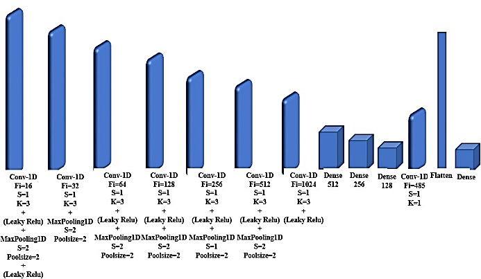
The suggested model of the CNN will be described in depth and depicted in Figure 7, which will outline the model's 26 layers: Eight 1D convolutional layers for feature extraction, seven leaky rectified linear unit, or leaky ReLU, six Max-Pooling 1D layers, four fully connected layers that represented by (Dense), and one flattens layer.
3.7. Performance measures
A range of measures were employed to assess the system's performance.
Precision: this measure is the quantity of the true positive elements divided by total number of the true positive elements and false positive cases. False positives are instances of the model which precisely label something as positive but are actually negative or, in this example, categorized as terrorists (Xiao et al., 1987).
Where TP: true positive and FP: false positive cases.
Recall: the ratio of data points which have been significant in this model indicates that such measure is the capacity to find all of the pertinent examples in a data set.
F-measure: The measure of precision, which is known as F (or F-measure) is utilized in the test for determining the grade. Accuracy of p is defined as the number of successful results divided by the total number of positive outcomes, while retrieval r is defined as the number of the positive cases divided by total number of the positive results. The harmonic intermediate accuracy and recall value is FF (mean F-1), where F-1 is the optimal at one and the worst at 0. Since general formula requires a true positive β, the F-score determines the accuracy regarding the recovery efficacy for a user who hangs β important times (Ghannay et al., 2018).
3.8. Client side
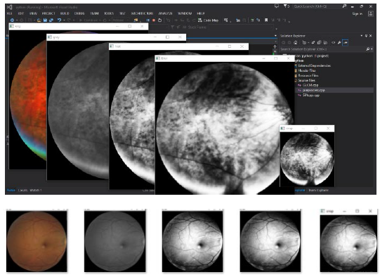
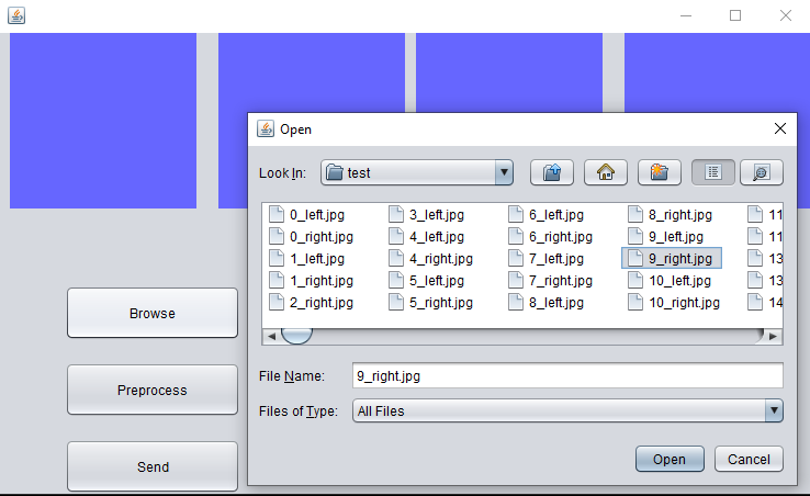
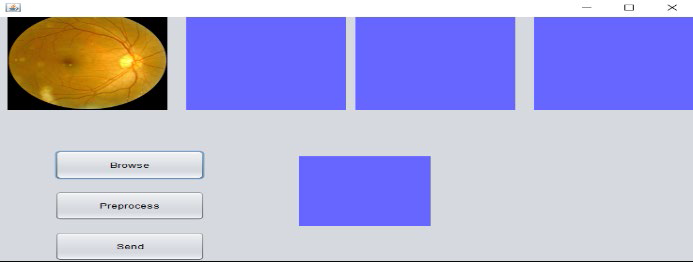
The first step in this aspect to carry out the work was to read the specific image. Figure 8 shows the main interface of the suggested system on the client side.

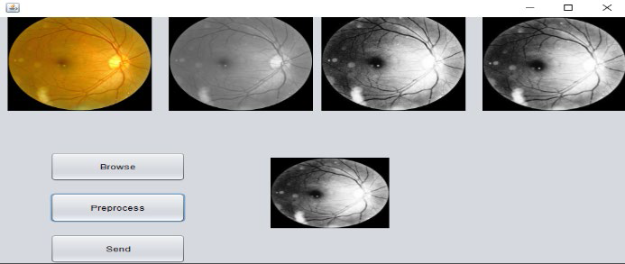
Figure 9 shows how to load the image from the dataset.
After that, the image has been pre-processed to be improved and get the best results. Figures 10 and 11 show the phase of conversion to gray level, the results of the histogram equalization for gray images and the result of resizing.
3.9. Server side
The Figure 12 shows how the image will be classification in the server side and then sent to the client.

4. Results and discussion
Results are shown in the presented section following the data-set's division into training and testing, with 70% toward training and 30% going toward testing. In order to achieve overall prediction results and display the system (Net Beans V. 8.0.2, for Java programming codes), DL is applied in Python IDLE (V. 3.6.5) following pre-processing and feature extraction operations (in Microsoft VS Ultimate 2013).
As it has been illustrated in Table 1, the results show that the best accuracy was achieved when the CNN algorithm that was applied to dataset (ODIR dataset) was 99.9% Recall, 99.9% precision and 99.9% F1-measure. Hence, the proposed diagnosing deep CNN model can be considered a successful model to diagnose the diseases.
Table 1 Classifier’s performance
| Classification algorithm |
Precision | Recall | F1-measure |
| CNN | 99.9% | 99.9% | 99.9% |
The study by Adio et al. (2011) examined the diagnosis of eye diseases in children in a teaching hospital in Nigeria. Although it provided a comprehensive overview of common diagnoses in a specific setting, it relied on traditional clinical examination and did not use machine learning or neural network techniques. In comparison, our study is more advanced in terms of using AI techniques to improve diagnostic accuracy while the study of Badah et al. (2023) investigated the use of machine learning techniques and neural networks to automatically diagnose eye diseases. While their study achieved good results, our study was distinguished by achieving significantly higher accuracy using the CNN model, which enhances the effectiveness of our model in diagnosis.
The study by Gour and Khanna (2021) used transfer learning in convolutional neural networks to detect multiple eye diseases. It has shown good results as well, but the 99.9% performance we achieved in our study outperforms most published results, showing that our model can be more effective in practical applications.
The study of Elfarra and Abuhaiba (2012) dealt with the diagnosis of breast cancer using computer-aided diagnostic systems and obtained noteworthy results in this field. Although it did not focus on eye diseases, it shows how important it is to use computing technologies to improve medical diagnosis in general. While our study is in line with this trend, it adds value by focusing on the use of CNN to diagnose eye diseases with superior accuracy. The results indicate that the proposed model can be considered a powerful tool for diagnosing eye diseases, as it outperformed many previous studies. This study provides evidence that small improvements in CNN model design and data selection can lead to significant improvements in performance, opening the door to further research to improve the accuracy of models applied in diagnosing various diseases.
In the context of comparing and discussing the results of our study with other references, it is possible to review the following points:
The study by Guergueb and Akhloufi (2021) examined the use of modern deep learning techniques to detect eye diseases. Promising results have been achieved using different techniques. However, we find that our study using a convolutional neural network (CNN) achieved better performance in terms of precision, recall, and F1-measure, suggesting that improvements in network design and data processing can lead to a significant improvement in performance. The study by Khan et al. (2022) focused on using deep learning to recognize eye diseases, while addressing the balance of internal classes in the data. Although the study provided performance improvements by addressing data balance, our study achieving 99.9% accuracy shows that using an efficient CNN model can outperform even without the need for advanced balance techniques, providing a simpler and more effective solution and the study by Li et al. (2022) used attention and feature fusion mechanisms to classify multi-label retinal images, yielding accurate results. However, the exceptional performance of our model shows that using techniques such as CNN may provide alternative solutions capable of achieving high levels of classification accuracy, even in multi-label scenarios.
The results achieved in our study show that the proposed CNN model outperforms many previous studies, both in terms of precision, recall, and fit score (F1-measure). This significant improvement reflects the high effectiveness of deep models in diagnosing eye diseases accurately and reliably. This comparison highlights the importance of recent advances in deep learning and advanced techniques such as attention mechanisms and feature fusion, which although effective, the model used in our study shows that distinct results can be reached even using relatively simpler techniques. This opens the door to the development of other models based on neural networks to target different types of medical data and achieve tangible improvements in different diagnostic fields.
5. Conclusions
In the presented paper, the model was used for predicting if an eye has a healthy fundus or an illness and to classify the major ocular diseases. 5,000 images representing eight distinct fundus types are included in the ODIR dataset. These classes represent the various ocular disorders, which were categorized with the use of DL models, like CNNs. Furthermore, the performance was much beyond expectations. The TensorFlow framework serves as the model's backend. This approach produced recall, precision, and F1 values of 99.9%, 99.9%, and 99.9%, respectively, during testing on the test images. A technique like this will transform the diagnosis of eye diseases and be very beneficial to medical practitioners. We think there's a chance for enhancement with further study and research in the near future, and that it might still be a valuable model. Images of additional forms of fundus disorders, particularly rare diseases in clinics, will eventually be able to be classified. This kind of challenge is challenging because small sample data classification has a low training effect. The way these illnesses are classified, nevertheless, is better suited for clinical use.

