1. Introduction

Coherent optical fiber communication (OFC) systems are usually used to transmit high-data rates over long-haul fiber transmission link (^{Neves et al., 2023}; ^{Escobar-Landero et al., 2023}). At the transmitter side, the input binary data is embedded in the amplitude A, phase ∅, or both, of the optical carrier. This carrier is presented by the electric field e(t) = Acos (2πω0t + ∅) emitted from a continuous-wave (CW) laser, where ω0 is the optical carrier (laser) radian frequency. This generally leads to three types of signal modulation formats, namely amplitude-shift keying (ASK), phase-shift keying (PSK), and quadrature-amplitude modulation (QAM), respectively, (^{Yang, 2021}). The QAM signal can be considered as the sum of two ASK signals which use the in-phase (I) and quadrature-phase (Q) components as their own optical carriers (i.e., cos(2πω0t) and sin (2πω0t), respectivelyT) (^{Binh, 2015}). he QAM digital signal element (i.e., symbol) can be expressed as (^{Binh, 2015}).

where aj and bk are bipolar discrete electric field amplitudes with j = 1, 2, … and k = 1, 2, … . The combination of the discrete amplitude sets {aj, bk} gives M discrete symbols, each has its own amplitude Aq = (aj2+bk2)1/2 and phase ∅q= tan-1(bk/aj). Here, q = 1, 2, …, M, and each one of the M symbols carries Log2 M bits of information. Thus, the M-QAM symbol has 4, 6, and 8 bits when M = 16, 64, and 256, respectively. A good graphical representation of the M-QAM signal is the constellation diagram (i.e., IQ-plane) which shows all the possible transmitted symbols as a collection of points (^{Haroun, 2023}). Each symbol is presented by a single point with the distance from the origin and the angle with respect to the I-axis representing the symbol amplitude and phase, respectively. Figures 1 (a) and (b) show the constellation diagrams of conventional 16-QAM and 64-QAM signaling, respectively. Note that in conventional communication systems (including OFC systems), the M-QAM symbols are transmitted with equal probability(=1/M).

Figure 1 Constellation diagrams of (a)16-QAM signaling and (b) 64-QAM signaling (^{Haroun, 2023}). 

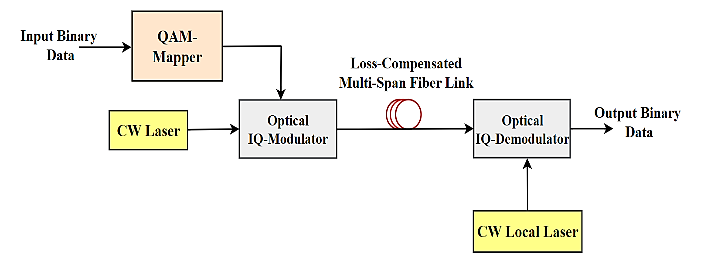
The coherent OFC systems usually use coherent detection to recover the data at the receiver side (^{Binh, 2015}). Here, the received signal electric field is mixed with that of a local CW laser whose frequency, phase, and polarization match those of the unmodulated transmitter laser. Figure 2 shows a simplified block diagram of an optical QAM communication system. The input binary data is converted to QAM symbols by the QAM mapper and then used to modulate the transmitter laser field. For long-haul transmission, the fiber link is constructed using multi-span configuration with each span consisting of a section of a single-mode fiber (SMF) followed by an optical amplifier to compensate the span loss (^{He et al., 2023}). Thus the transmission link acts as a quasi-lossless channel. At the receiver side, the detected symbols are converted back to binary data using QAM demapper. The propagation of the QAM symbols in the fiber is influenced mainly by fiber material dispersion, as a linear effect, and nonlinear fiber optics (^{Liang et al., 2023}). This nonlinearity effect increases in WDM systems where a group of OFC systems uses the same fiber link (^{Deligiannidis et al., 2023}). The nonlinear fiber effects and their interaction with fiber dispersion lead to nonlinear interference (NLI) which plays a key role in determining the bit rate-distance product in WDM-OFC systems. This issue should be addressed carefully in these advanced communication systems.

Figure 2 Simplified block diagram of an optical QAM communication system. 

Recently, there is increasing interest in using constellation shaping (CS) techniques to reduce the effect of NLI in WDM-OFC systems (^{Civelli, 2024}; ^{Xing et al., 2024}). These techniques are classified into three categories, namely geometric constellation shaping (GCS), probabilistic constellation shaping (PCS), and joint GCS/PCS (JGPCS) (^{Liu et al., 2023}). In GCS, the locations of the points in the constellation diagram are rearranged without changing the probability of the symbols (=1/M) (^{Xing et al., 2024}). The PCS technique changes the probability of the symbols without affecting their power (i.e., their locations in the constellation diagram) (^{Amirabadi et al., 2022}). The JGPCS combines the effect of both GCS and PCS techniques (^{Yao et al., 2023}). In CS-assisted OFC systems, the conventional QAM mapper (demapper) is modified to produce (deals with) a new constellation diagram by encoding (decoding) the binary data according to the used CS technique. Therefore, the modified mapper and demapper are called encoder and decoder, respectively. The use of the deep learning (DL) technique in the design of these two components DL attracts increasing interest in recent years. These two components can be designed synchronously using end-to-end deep learning (E2EDL) techniques and therefore, they are lumped as one virtual component called autoencoder (AE). The performance of the E2EDL-based GCS-WDM system has been investigated by some research groups assuming five multiplexed channels (^{Jones et al., 2018}; ^{Jones et al., 2019}; ^{Oliari et al., 2021}; ^{Jovanovic et al., 2022}), and (^{Jovanovic et al., 2023}), 11 multiplexed channels (^{Gümüs et al., 2020}), and more number of channels (^{Abbass & Fyath, 2024}).

The model-driven simulation approach is constructed in a divide-and-conquer manner and consists of a series of model blocks (^{Wang et al., 2020}). Among these models are laser, pulse shaper, modulator, fiber channel, optical amplifiers, filters, and detectors. All these blocks are characterized by rigorous numerical models (^{Wang et al., 2020}). Commercial optical communication software is usually non-open and the expensive (^{Jiang et al., 2022}). Furthermore, computation complexity of conventional simulations can be very high due to the nested-function construct and the repeated iterative operation (^{Jiang et al., 2022}). For example, the optical fiber channel can be modeled using the split-step Fourier method (SSFM). This method is based on solving numerically the nonlinear Schrödinger equation (NLSE) which describes pulse

propagation in the fiber and takes into account both linear and nonlinear fiber effects. In this method, the optical fiber is divided into multiple short-length segments (steps), and the fiber linearities and nonlinearities are calculated separately for each step (^{Yang et al., 2022}). Using a shorter-step distance offers high modeling accuracy but requires a large computation time. To reduce the computation time, a data-driven proposed to characterize the transmission in OFC systems (^{Neves et al., 2023}). In this model, the fiber channel is replaced by an ANN which is trained by data collected from experimental measures or from first-step simulation predictions. This modeling approach applied successfully for single-channel (^{You et al., 2023}) and multi-channel (^{Yang et al., 2022}) OFCs. The investigation in these references focuses on comparison with the model-driven approach and to select the suitable ANN configuration for that purpose. However, no DL-based data-driven optical fiber channel modeling is reported in the literature for constellation shaping-assisted OFCs even with the single-channel operation. This issue is addressed in this work where a flexible ANN-based fiber modeling is proposed which can be applied to GCS, PCS, and JGPCS WDM-OFC systems.

2. Related works

In 2020, ^{Wang et al. (2020)} proposed a data-driven modeling approach utilizing bidirectional (Bi)-long short-term memory (LSTM) NNs to mimic fiber channel. Both on-off keying and pulse amplitude modulation-4 signals were studied for transmission. The Bi-LSTM-based method demonstrated strong performance and produced results comparable to the conventional SSFM-based model. In 2022, ^{Jiang et al. (2022)} Investigated data-driven approach utilizing a deep neural network (DNN) to predict the nonlinear fiber channel in OFC systems. The DNN method effectively represents the transfer function of the fiber channel. In 2022, ^{Yang et al. (2022)} suggested a hybrid model-data-driven approach for rapid and precise waveform modeling of long-distance multi-channel optical fiber transmission. It utilizes a linear-nonlinear feature decoupling distributed waveform modeling technique. The conventional approach used for modeling waveforms in optical fiber communication systems is the SSFM. In 2023, ^{You et al. (2023)} suggested a method for modeling optical fibers with low complexity LSTM (C-LSTM), and the computational complexity of C-LSTM was determined for comparison with modeling techniques based on conditional generative adversarial networks and SSFM.

The ANN-based end-to-end deep learning technique have been investigated in the literature. Table 1 presents a comparison between some of these works and the one reported in this paper.

Based on the previous survey, it is obvious there is no document reported in the literature that uses DL-based data-driven optical fiber channel modeling for CS-assisted WDM systems to achieve high-capacity data transmission. To achieve this issue, this work presents a flexible ANN-based fiber modeling approach that is applicable to these systems.

3. General algorithm of multi-span optical fiber modeling-based artificial neural networks

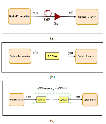
Figures 3 (a)-(c) explain the block diagrams of the main steps to design general multi-span optical fiber model-based ANNs, and the steps are stated below:

Step I: Data collection

Simulate the OFC system assuming a single-span transmission link. Choose a specific fiber channel model in the simulation (such as NLIN or SSFM) and record both the input and output data of the fiber ( x(t) and y(t)).

Step II: ANN training

Choose ANN configuration and train it to model a single-span transmission link system. Train this network, ANN-single span (ss), using the data collected in step I.

Step III: Construction of the multi-span link modeling

The ANN model of the multi-span (ANN-ms) link is constructed by Nsp of ANN-ss where Nsp is the number of spans.

Figure 3 Block diagrams of general multi-span optical fiber modeling-based ANN. (a) data collection, (b) ANN training, and (c) construction of the multi-span link modeling. SMF: Single-mode fiber, OA: Optical amplifier. 

4. Optical fiber communication channel model using ANNs

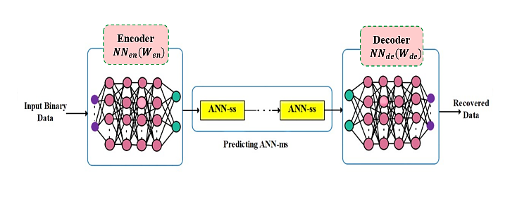
The configuration of the communication system and the alternative approach for modeling the OFC using an ANN are illustrated in Figure 4. In this figure, the AE simulation platform comprises two NNs positioned in the encoder and decoder, with a fiber channel model connecting them.

Figure 4 AE simulation platform with optical fiber modeling of ANN-ss. 

The modulated carrier x(t) is transmitted across the OFC channel to produce an output y(t).

The NLIN channel model, fNLIN, investigates the impact of nonlinear interference on fiber communication (^{You et al., 2023}). To account for the nonlinear effects that degrade the broadcast signal, this model considers the launch power per channel as well as the constellation's moments. The NLIN model simplifies these nonlinear effects into additive white gaussian noise (AWGN), with the variance controlled by the fiber communication channel parameters. As a result, the channel impairments are controlled by the amplified spontaneous emission (ASE) noise, which is dictated by the amplifier noise figure Fn, the average launch power per channel (referred to as launch power), and the constellation's high order moments (^{You et al., 2023}).

The noise variance can be calculated as follows

where σASE2 Fn is the ASE noise variance, and σNLIN2 is the nonlinear interference variance which is a function PL, μ4, and μ6.

The encoder and decoder are both represented by dense layers, denoted as NNenwen for the encoder and NNde(wde) for the decoder. The variables wen and wde represent adjustable weights, including biases, that can be trained to enhance the performance of the system (^{Jovanovic et al., 2021}). The transmitted and the received symbols can be represented by tx =NNen (s,wen), and rx = NNde (s^,wde), respectively, the role of the encoder is to convert the input signals into sent symbols, aiming to minimize the effects of channel distortions. The decoder produces output signals often expressed as the posterior probability of the transmitted messages. Using these probabilities, the receiver can successfully recover the original input messages. When considering an AE for this system, the input of the encoder usually comprises a probability vector, which is sometimes referred to as a one-hot vector. This vector denotes the symbols that are being transferred. Each one-hot vector is represented as s ∈ S = {ei|i =1, ..., M}; where M denotes the modulation order and ei is a binary vector with all elements set to zero, save for a single '1' at position i, denoting the symbol's position (Zhang et al., 2022; ^{Srinivasan et al., 2023}). The AE model's encoder optimizes the positioning of the constellation points, while the decoder learns the decision limits of the distorted symbols (^{Jovanovic et al., 2022}).

The parameters for training the AE in this work are provided in Table 2. A total of 250 epochs were used. The Glorot initialization is employed to initialize the weights set (^{Rex et al., 2022}). During each epoch of training, a new set of samples is created. These samples consist of 𝑁 = 128 × 𝑀 one-hot encoded vectors that are evenly distributed. The vectors are then separated into batches of size 𝐵 = 16 × 𝑀. The learning rate is optimized to 0.001. The number of batches is determined by dividing the total sample size by the specified batch size. In order to classify, a softmax layer is employed at the decoder. The purpose of this layer is to convert the decoder's output into a probability vector, ensuring that the sum of its elements is equal to one (^{Cardarilli et al., 2021}).

The AE technique is founded on the principle of E2EDL, which aims for joint optimization of the components of the transmitter and receiver within a single process. Nevertheless, a significant limitation that obstructs the practical application is the requirement of a differentiable channel model, namely the knowledge of the gradient of the instantaneous channel transfer function. If the channel lacks a differentiable model, the gradients cannot be calculated during back-propagation to alter the network's parameters during training.

DL has the capability to approximate any function, and it can give an effective solution for linear and nonlinear problems. DL offers an innovative framework for reevaluating the optical communication modeling problem. DL models approximate the model functions by mapping independent variables to dependent variables that correlate to the input and output data (^{Wang et al., 2020}). Therefore, the ANNs are strategically used to define the segment located between the encoder and the decoder and to accelerate the training process of the E2EDL system. Firstly train the AE at a single span (ANN-ss) with a span length of 100 km and store the outputs and inputs of the encoder and decoder, respectively, these values represent the transmitted and received symbols. In this situation, the communication fiber channel consists of a conventional SMF, and to emulate the OFC, use the nonlinear interreference noise (NLIN) fiber model. This model is built upon an improved Gaussian noise model. It is described as an additive Gaussian noise process and assesses its variance and spectrum (^{Dar et al., 2013}; ^{Dar et al., 2014}). The erbium-doped amplifier (EDFA) is used at the end of the span to compensate for the loss of signal. The amplifier has a noise figure of 5 dB. This AE is designed based on a WDM system to increase data transmission capacity, and Table 3 lists the parameter values of the WDM system used in the AE platform.

After the AE training procedure is finished on a single span, the encoder and decoder input-output data are saved. Afterwards, the stored data are retrieved and used as inputs and labels to train Bi-GRU-NN (^{Liu et al., 2023}) and CNN (^{Jiang et al., 2023}) separately. This methodology is utilized to obtain an efficient ANN model that is specifically tailored for a single span, which is referred to as the ANN-ss model. The trained ANN-ss model is stored and retrieved to employ for substituting the conventional OFC (NLIN) model for single span and then used this model for predicting ANN-multi spans ANN-ms) by implementing the cascaded of the ANN-ss model and it is used as a replacement for the optical fiber spans in the communication system as shown in Figure 5. The ANN-ss model is configured in a cascaded manner to effectively simulate long-distance optical transmission systems using different numbers of WDM-channel systems at flexibility.

Figure 5 Optical Fiber modeling for ANN-multi-span link. 

The BER is a metric that calculates the probability of an error using the number of erroneous bits per transmitted bit (^{You et al., 2023}). The BER of the M-order modulation format is determined using (^{You et al., 2023}).

where M is the number of discrete symbols involved in the modulation (i.e. modulation order), m is the number of bits per transmitted symbol (m =log2M ), and erfc denotes the complementary error function.

5. Architecture perspectives: Artificial neural networks structures

In this section, describe the architecture of the proposed Bi-GRU-NN and CNN models, which are used for modeling the OFC in AE-based GCS-WDM system for long-haul transmission distance.

5.1. Bi-directional gated recurrent neural networks

This subsection provides a detailed explanation of the structure of the GRU and the proposed Bi-GRU-NN models, which are employed for optical fiber prediction. recurrent neural networks (RNNs) considered the sequence correlation can typically reconstruct the channel crosstalk in most situations (^{You et al., 2023}). In addition, RNNs are frequently used to identify connections in data that are arranged in a sequence and have temporal dependencies. This makes them particularly suitable for channel predicting. Among the several types of RNNs, the LSTM model is especially proficient at mitigating the problems of vanishing gradients and gradient explosion that are common in regular RNNs. GRU, a variant of LSTM, and GRU provides immunity for gradient explosion, and utilizes gated cells to control the flow of input within the network, resulting in a simpler implementation compared to LSTM. Meanwhile, GRU is a simpler variant of LSTM and uses gated cells to regulate the flow of information within the network, making its implementation easier than LSTM (^{Hu et al., 2023}).

Each GRU cell consists of two gates: an update gate and a reset gate. An update gate regulates the flow of control information into the following instant, while a reset gate controls the loss of information. These two gates together decide the output of the hidden state (^{Yin et al., 2021}). The structure of the GRU unit is explained in Figure 6, the GRU unit computes the ultimate result by considering the current input txt and the prior state h_t-1, taking into account the combined impact of these gates. A summary of the internal gate outputs of the GRU unit is provided below (^{Liu et al., 2023}).

rt= σ  Wr  ht-1, txt+ br

zt= σ ( Wz  [ht-1, txt] + bz)

h~t= tanh ( Wh  [rt⨀ht-1, txt] + bh)

ht= (1- zt) ⨀ht-1 + zt ⨀h~t (6)

where Wr, Wz and Wh denotes the weight matrices for the reset gate, the update gate, and the new calculation of the memory, respectively. The bias vectors br, bz, and bh relate to each other. The sigmoid function σ is used for both the reset and update gate. In the context of memory computation, the hyperbolic tangent activation function is denoted as tanh, while the Hadamard product is represented as ⨀.

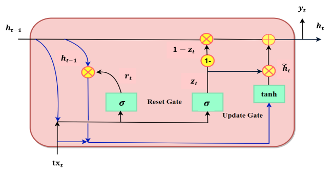
Figure 6 Diagram depicting the structural components of a GRU memory unit, edited from (^{Liu et al., 2023}). 

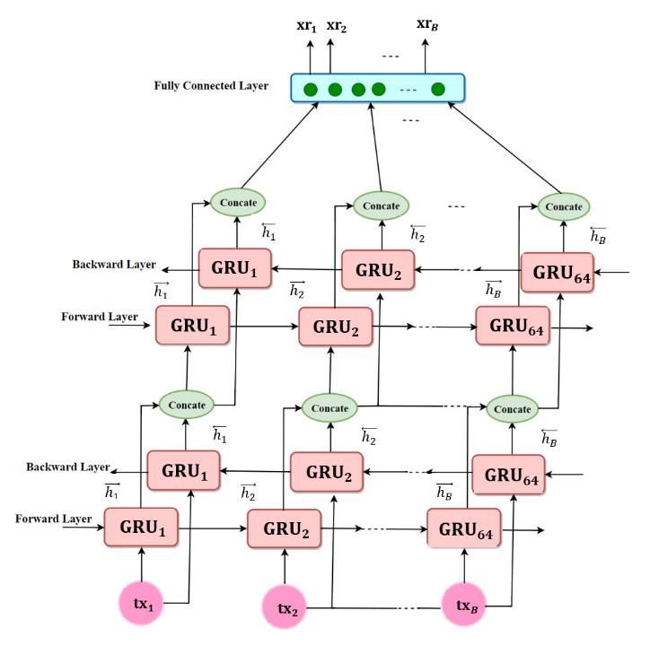
This work uses two layers of Bi-GRU-NN layers, A Bi-GRU-NN layer consists of 64-GRU units that process the input sequence in the forward direction and another 64-GRU unit that process in the backward manner. The bidirectional GRU helps mitigate the problem of error propagation resulting from unidirectional prediction. Furthermore, the bidirectional GRU approach enhances feature extraction precision by thoroughly examining the correlation between nearby data points. The output layer comprises a fully connected layer that employs a linear activation function to compute the weighted sum of the hidden layer outputs. The structure of the Bi-GRU-NN is illustrated in Figure 7.

Figure 7 Architecture of the Bi-GRU-ANN that is used for optical fiber modeling. 

5.2. Conventional neural networks

In the field of optical communication, CNNs are employed for various reasons. They are utilized for different tasks such as classification and serve as effective equalizers, exhibiting excellent bit error rate (BER) performance and possessing robust equalization capabilities (^{Musumeci et al., 2019}). In addition, CNN is used for modeling optical fiber communication which yields exceptional predictive accuracy (^{Jiang et al., 2023}). Therefore, this work uses CNN for modeling the optical fiber. This subsection provides a detailed explanation of the design of the CNN model, which is employed for optical fiber prediction in the AE-based GCS-WDM system.

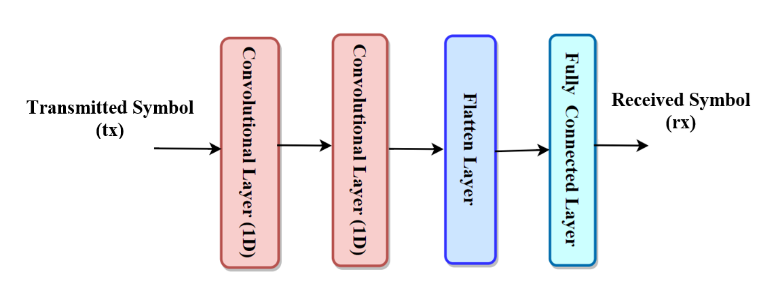
Figure 8 illustrates the architectural setup of the CNN model used in this work. The model consists of two layers of one dimensional (1D)-CNN that the transmitted symbols tx are applied to it, without using max pooling layer, followed by a flatten layer. The flatten layer serves the purpose of converting the output data into a flattened vector format, guaranteeing compatibility with the succeeding fully connected layer (FCL). The sequential structure of this model allows for efficient extraction of features using convolutional processes. These features are then transformed into a one-dimensional vector representation, which is suitable for the processing requirements of the FCL. The FCL is positioned at the end of CNN network architecture and is considered as an output layer and it receives input from the preceding convolutional layer. The provided input is a vector derived from the feature map after it has been flattened (^{Liu & Zhao, 2023}). The presence of a substantial number of trainable parameters makes the FCL layers necessary to accommodate intricate nonlinear discriminant functions in the feature space, where the input data pieces are transformed (^{Basha et al., 2020}).

Figure 8 Architecture of the CNN that is used for optical fiber modeling. 

5.3. Comparative analysis: Bi-directional gated recurrent neural networks vs. convolutional neural networks

This section presents a performance comparison of the AE-based GCS- WDM system using both Bi-GRU-NN and CNN modeling architectures. Both models undergo training for a total of 150 epochs. The weights set is initialized using the Glorot initialization approach, which guarantees an efficient initialization of network weights to facilitate optimum learning during training (^{Rex et al., 2022}). The batch size equals 1024 for each model. When it comes to regression, the MSE is a reliable assessment metric for assessing the quality of an estimator. It takes into account both the variance and bias of the estimator. Therefore, the MSE is chosen as the assessment indication and a highly effective performance (^{Wang et al., 2020}). The MSE in this work represents the mean of the squared amplitude errors, which is the average of the squared differences between amplitude values of the NN-ss produced and the NLIN-generated waveforms. The normalized MSE is used to statistically assess the similarities between the two simulation approaches. Given the simulation of optical communication systems using various optical launch powers, it is seen that the absolute MSE may grow with higher power levels. Therefore, instead of using the absolute MSE, the normalized MSE is preferred. The normalized MSE is defined as follows (^{Jiang et al., 2022})

MSE_norm =∑im(Y--Y)2∑imY-2 (7)

where m denotes the sample size, Y- represents the output label (i.e., rx) signal and the output signal generated by the ANN-ss is Y.

A comparison of the normalized MSEs of the ANN-ss versus epoch numbers between Bi-GRU-NN and CNN is shown in Figs. 9 (a) and (b). For DP 64-QAM, baud rate (R _s ) = 40 Gbaud, the launch power (P _L ) = -2 dBm, and the number of channels N _ch (a) = 32, (b) = 64. The normalized MSEs for both ANN models reach low levels of 10^-3. More precisely, when N _ch is equal to 32 and 64, the Bi-GRU-NN model exhibits normalized MSEs of 3.64x10^-3 and 3.90x10^-3 respectively. By comparison, the normalized MSEs of the CNN for the identical channel topologies are 3.81x10^-3 and 4.51x10^-3. As a result, the ANN-ss of Bi-GRU-NN shows smaller losses in comparison to CNN.

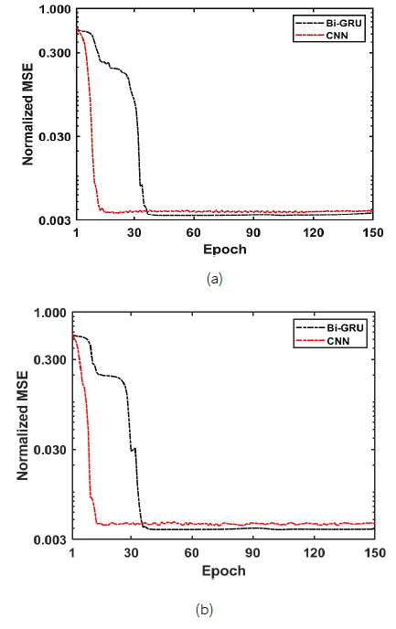
Figure 9 Variation of the normalized MSE of the ANN-ss with epoch numbers for Bi-GRU-NN and CNN, DP 64-QAM, respectively. N_ch (a) = 32, (b) = 64, and P_L = -2 dBm. 

Figures 10 (a) and (b) depict a comparison of the AE-based GCS-WDM system performance using the NLIN model, ANN-ms using Bi-GRU-NN and CNN for various values of spans at N _ch (a) = 32, (b) = 64, R _s = 40 Gbaud, and P _L = -2 dBm in terms of BER as a function of the number of link spans, respectively. It is evident from these figures that the BER of the three systems is comparable at a small number of spans and gives BER values below the BER threshold (BER _th ) for the different number of spans. The performance of the developed AE-based GCS-WDM system is enhanced in terms of BER when Bi-GRU-NN is used to model the multi-span fiber link (i.e., the system response has a lower BER than when CNN is used to model the multi-span fiber link for the 32 and 64 channels). While an AE-based GCS-WDM system was devised, it was determined that modeling the multi-span fiber link with CNN yields a more comparable BER to the optical fiber link. Tables 4 (a) and (b) provide a comparative analysis of the AE's performance when trained using the same system parameters given above, which lists BER for various values of the results demonstrate that the AE-based GCS-WDM system using the Bi-GRU-NN model gives better performance across various N _sp values. The simulation results reveal that the data-driven (ANN) model reduces computation time by approximately 7% compared with the numerical NLIN model, and this time reduction is almost independent of the used ANN configuration and number of spans.

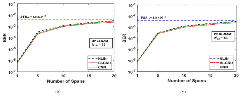
Figure 10 Variation of the BER with a number of spans for AE-based GCS-WDM system performance for DP 64-QAM using NN-multi-spans of Bi-GRU-NN and CNN for various values of spans. N _ch (a) = 32, (b) = 64, and P _L = -2 dBm. 

Table 4 Comparison of AE-based GCS-WDM system performance using NLIN model, NN-multi-spans for Bi-GRU-NN and CNN for various values of spans in terms of BER, assuming DP 64-QAM and P _L = -2 dBm. (a) N _ch = 32 (b) N _ch = 64. 

Channel Model	Bit Error Rate (BER)
	Number of Spans Nsp
	1	5	10	15	20
Fiber (NLIN)	7.23 x 10-7	3.32 x 10-4	1.24 x10-3	2.19 x 10-3	3.31 x10-3
Bi-GRU-NN	6.01 x 10-7	2.15 x 10-4	9.80 x 10-4	1.72 x 10-3	2.36 x 10-3
CNN	6.53 x 10-7	2.53 x 10-4	1.09 x10-3	1.94 x 10-3	2.96 x 10-3
(a)
Channel Model	Bit Error Rate (BER)
	Number of Spans Nsp
	1	5	10	15	20
Fiber (NLIN)	8.03 x 10-7	3.34 x 10-4	1.26 x10-3	2.22 x 10-3	3.35 x 10-3
Bi-GRU-NN	7.24 x 10-7	2.56 x 10-4	9.85 x 10-4	1.65 x 10-3	2.52 x 10-3
CNN	7.72 x 10-7	2.94 x 10-4	1.14 x 10-2	1.95 x 10-3	3.11 x 10-3
(b)

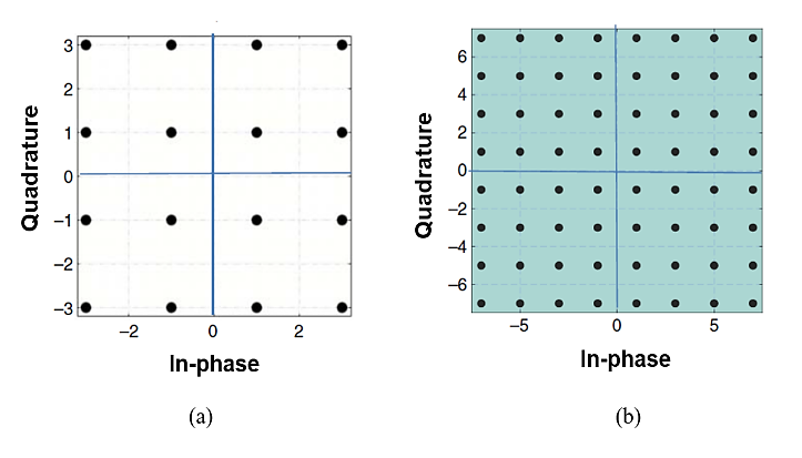
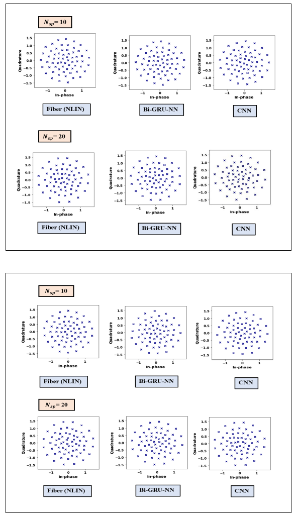
Figures 11 (a) and (b) display the learned constellation diagrams for N _sp = 10 and 20 for N _ch (a) = 32, (b) = 64, R _s = 40 Gbaud, and P _L = -2 dBm. Using NLIN model, NN-ms for Bi-GRU-NN and CNN. These figures show that the distribution of constellation points in the constellation diagrams at 10 spans is nearly identical for all three models at N _ch = 32, and = 64, respectively, and these points are arranged in regular rings and uniform distribution, which indicates a low BER. While at 20 spans, leading to a greater BER, it is observed that the locations of the inner symbols slightly change so long as the BER remains below the BER _th but the outer rings remain uniform. However, the better arrangement of the learned constellation of AE is by using the Bi-GRU-NN model that gives lower BER. Furthermore, it is observed that the constellation has been learned to tolerate NLI noise.

Figure 11 Learned constellation diagram at different numbers of spans for AE-based GCS- WDM system, assuming N _ch (a) = 32, (b) = 64, N _sp = 10, and = 20, R _s = 40 Gbaud, and P _L = -2 dBm for DP 64-QAM. 

6. Conclusion

A versatile ANN-based low-computation model has been developed for optical fiber channel in WDM systems. The model has been applied successfully to a case study incorporating E2EDL-based GCS WDM systems designed with multi-span transmission link. The simulation results reveal that the data-driven (ANN) model reduces computation time by approximately 7% compared with the numerical NLIN model, and this time reduction is almost independent of the used ANN configuration. Further, The performance of the developed AE-based GCS-WDM system is enhanced in terms of BER when Bi-GRU-NN is used to model the multi-span fiber link for the 32 and 64 channels. While an AE-based GCS-WDM system was devised, it was determined that modeling the multi-span fiber link with CNN yields a more comparable BER to the optical fiber link. The better arrangement of the learned constellation of AE is by using the Bi-GRU-NN model that gives lower BER. Furthermore, it is observed that the constellation has been learned to tolerate NLI noise.