nueva página del texto (beta)
 Inglés (pdf)
 Artículo en XML
 Referencias del artículo
 Enviar artículo por email
 Citado por SciELO
  Similares en
SciELO
Similares en
SciELO 
 Permalink
1. Introduction
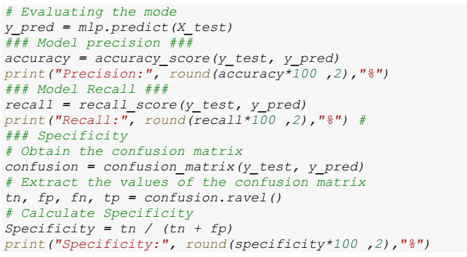
Dengue, caused by the dengue virus transmitted by Aedes aegypti mosquitoes (Figure 1), represents a global threat in more than 125 countries in tropical and subtropical regions. Annually, approximately 390 million cases are reported worldwide, with 96 million manifesting clinical symptoms. (Thomas et al., 2022). The disease is not limited to tropical areas, as cases have been reported in the southern U.S. and in some European countries such as Italy, France, Greece, and Spain. (Mattar et al., 2019).
The diagnosis of dengue is made through laboratory techniques, such as dengue-specific polymerase chain reaction with reverse transcription (PCR-RT), detection of the "non-structural" protein (NS1), evaluation of Immunoglobin type M- IgM, Immunoglobin type M - IgG, and virus isolation. In addition, clinical signs and symptoms play a vital role in the differential diagnosis. (Rubiano Godoy & Jiménez-Cendales, 2021)
Dengue (DENV) is part of a group of viruses known as the dengue serocomplex. It belongs to the genus Flaviviridae. The dengue serocomplex has different serotypes of different viruses: dengue type 1, 2, 3 and 4. They share similarities in structure and pathogenicity. In areas where dengue is common, all four virus serotypes circulate regularly in both endemic and highly endemic areas. These serotypes do not differ significantly from each other, as they are all capable of causing the disease known as dengue. This disease is of a viral nature and is entrenched in these regions. (Vargas-Navarro et al., 2021).
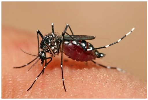
Dengue infection has a variety of clinical manifestations shared by other vector-borne viral infections, such as Chikungunya and Zika: (Figure 2).
Fever: Common symptoms of dengue fever last from 2 to 7 days.
Arthralgias: Pain in the joints is intense and limiting.
Myalgias: Pain in the muscles, intense and limiting.
Headache: May be severe and persistent.
Maculopapular rash: The skin may present the appearance of areas with red spots, which may vary in shape, some being flat and others with a small elevation.
Conjunctivitis: It is the inflammation of the conjunctiva, it may cause redness, itching and tearing.
Lymphadenopathy: Enlarged lymph nodes, which may be painful to the touch.
Leukopenia: A reduction of white blood cells in the blood and this may increase the chance of further infections.
Thrombocytopenia: A decrease of platelets in the blood increases the likelihood of experiencing bleeding.
Asthenia and Adynamia: Perception of weakness and lack of energy. (Rubiano Godoy & Jiménez-Cendales, 2021).
A complete diagnosis of dengue requires a complete medical evaluation.
According to WHO, it is divided as follows:
Outpatient treatment: Mentions patients with non-severe cases of dengue, where actions are implemented to manage the signs and symptoms. Self-care is promoted, avoiding self-medication, maintaining adequate hydration, and visiting the nearest health center to monitor temperature and vital signs.
Hospital treatment: Mentions the need for hospitalization of patients with hepatomegaly, hypotension, lethargy, increased capillary permeability, plasma leakage, dehydration, signs of shock and bleeding.
Intensive care: Depending on the severity of the clinical condition, the patient may require admission to an intensive care unit, where complications such as encephalitis, myocarditis, liver enlargement, fluid accumulation in the abdomen, fluid accumulation in the lungs (pleural effusion) and multiple organ failure may occur.
One of the ways to prevent is to avoid the formation of breeding sites, which reproduce in areas where water accumulates frequently. This is achieved by eliminating expendable objects that contain stagnant water, it is also recommended to cover well the tanks that contain water. It is important to keep yards and gardens tidy, weeded, and clean.
It is also suggested that people wear long sleeves and long pants and always use repellent.
In this context, the present research aims to compare different machine learning algorithms to develop an effective classification model for the identification of dengue virus cases. The application of machine learning algorithms in the field of health has become essential, allowing us to analyze complex data more efficiently than traditional modeling methods. (Yang Santos et al., 2023)
This research is of vital importance to increase the accuracy of diagnosis and promote timely treatment, optimizing the use of resources and contributing to scientific progress.
Previous studies, such as that of (Shaikh et al., 2023), highlight the usefulness of algorithms such as random forest and LightGBM for early prediction, providing accuracies of 76.9% and specificity of 87.9% at the plasma escape stage in dengue patients. Consistent with previous research, our work is framed for dengue case prediction and classification. The research of (Yang et al., 2023) highlights the value of random forest in identifying complex patterns and predicting 43.1% of severe cases. Other studies, such as (Handari et al., 2021), use methods such as Long Short-Term Memory (LSTM) to predict cases of dengue hemorrhagic fever with high accuracy. The Long Short-Term Memory (LSTM) method excelled with an accuracy of 0.04427%, offering the best predictions of cases in DKI Jakarta. These results are valuable for health authorities in the prevention and control of future outbreaks. Likewise, (Yavari Nejad & Varathan, 2021) state that they want to predict dengue outbreaks and improve accuracy with machine learning. They evaluated five models, highlighting a Bayesian network with a new risk factor, reaching 92.35% prediction accuracy. They conclude that identifying factors improves the prediction of dengue outbreaks, similarly, (Lim et al., 2020) explain that they wish to predict dengue epidemics through Bayesian regime shift models, using algorithms such as BAR and BRS. The BRS model demonstrated a higher predictive ability than time series models, identifying the influence of climatic factors on dengue transmission, with a MAPE of 5.43%. It is concluded that the regime shift models were more suitable for understanding the dynamics of dengue transmission, suggesting their value in epidemiology. In turn, (Li et al., 2022) say they seek to improve the accuracy of dengue case predictions with limited time series data. They used the Earth Engine (GEE) platform and the LSTM model to achieve this, obtaining a low mean square error (0.33%) and mean absolute percent error (0.28%) at week 12. This approach has great potential to forecast dengue risk effectively and practically, and its application in other regions or globally is suggested to strengthen disease prevention and control strategies, also, (Tanawi et al., 2021) note that they focus on predicting dengue cases in DKI Jakarta using climatic and previous data. Support vector regression models with linear and radial kernel were compared, with the linear being more accurate with a mean square error of 3.6678%. Variables such as temperature and cumulative rainfall correlated positively, while mean temperature correlated negatively, highlighting the influence of climate on dengue cases, furthermore, (Kaur & Sharma, 2023) argue that they wish to predict and diagnose dengue using various machine learning algorithms in Python. Where DT, CART and NB showed higher accuracy, sensitivity, specificity, and recall. A model that predicts dengue infection based on vital signs and symptoms was developed with greater than 90% accuracy and 90% accurate classification rate. Machine learning algorithms can extract hidden patterns in dengue data for accurate detection and improve disease management, finally, (Hamdani et al., 2022) that they seek to classify dengue patients using machine learning and symptoms as data, they compared algorithms such as KNN, RF, DT and SVM, finding that SVM was the most effective with 99.1% accuracy, recall and precision. They concluded that machine learning can be highly effective in diagnosing and predicting the type of dengue based on symptoms, which is crucial for proper treatment and early detection.
In this context, the present research contributes to the field by focusing on the comparative evaluation of algorithms, incorporating both technical aspects such as attribute selection and data partitioning. In addition, it seeks to identify specific patterns related to dengue, contributing to the growing understanding of this disease. The need for accurate classification of dengue cases not only has medical implications, but also extends to efficient resource management and informed public health decision making. The conclusions derived from this research could be essential to inform more effective health policies and prevention strategies, providing a solid foundation for future research in this field.
2. Materials and methods
Several essential resources were used to conduct the investigation. First, a dataset containing clinical information on 21,157 individuals presenting with dengue symptoms was used. This dataset, composed of truthful information, was essential to conduct a detailed analysis.
As for the development platform, Google Colab was chosen, which provides free access to computational resources. This platform not only facilitates real-time collaboration, but also includes pre-installed libraries, creating an efficient and accessible development environment.
For the execution of the analysis, a laptop with an Intel Core i5-1135G7 11th generation 2.40 GHz processor, 8.00 GB of RAM and Windows 10 operating system were used.
The programming language selected was Python, recognized for its specialized machine learning libraries. In addition, the clear and readable syntax of Python facilitated the development of the code, improving the understanding and interpretation of the results obtained in the study. Together, these elements formed the necessary technical basis for the research, enabling efficient and effective analysis of dengue-related data.
2.1. Dataset
In the first instance, it was necessary to build a dataset with which the machine learning algorithms should be implemented. It was considered essential to collect information from reliable sources in the department of Lambayeque, specifically in the field of public health. The focus was on collecting real and relevant data on dengue cases that have occurred in the first months of the year. This path was followed because, although there are datasets related to dengue available in platforms such as Kaggle and others, many of them are linked to data that are not relevant to this research. However, the interest lies in working with specific clinical data within the Lambayeque region.
Data collection was conducted in a public hospital, following strict confidentiality and privacy protocols. This approach guaranteed the construction of a reliable and valuable database, fundamental for the development of research. The creation of the dataset was governed by rigorous criteria to ensure accuracy and relevance in the information collected. These criteria are detailed below:
Period: Refers to data collected during the months of January to July 2023. This choice is based on the observation that there was a significant increase in the number of dengue cases during this period.
Outcome: The data used in this field are divided into two main categories: "confirmed" and " discarded". These results are obtained from the tests performed on patients, which allows for accurate classification of dengue cases.
Age: People were classified into age groups following the technical regulations established by the Ministry of Health in Peru. These groups are:
Sex: Dengue cases were classified into two categories: Female and male, to analyze the differences in the incidence of dengue according to gender.
Symptoms: Dengue-related symptoms were considered. These symptoms can vary in severity, from mild to severe, and even life-threatening in some cases. Typical symptoms of dengue usually manifest 4 to 10 days after the bite of an infected mosquito considering fever, headache, eye pain, bone pain, nausea, and rash.
Imported: We have considered dengue cases contracted outside the Lambayeque region, which allows us to analyze the spread of the virus from other areas.
Autochthonous: We have considered dengue cases that originated within the Lambayeque region. This is essential to understand the local dynamics of the disease and its impact on the community.
After establishing these criteria, we proceeded to the selection and collection of relevant data. Table 1 shows that the result was a robust and representative dataset with 21,157 cases, including confirmed and discarded cases. It was then transformed into a .csv format to facilitate model training and perform advanced analyses, thus ensuring the quality and usefulness of the dataset for research. This meticulous approach to dataset construction supports the robustness and relevance of the results obtained in the study.
Table 1 Dataset structure.
| Period | Outcome | Age | Sex | Symptoms | Imported | Autochthonous | |||||
|---|---|---|---|---|---|---|---|---|---|---|---|
| Fever | Headache | Eye pain | Bone pain | Nausea | Rash | ||||||
| January | confirmed | 18_29 | Female | Yes | Yes | Yes | Yes | No | Yes | Yes | No |
| January | discarded | 0_11 | Female | Yes | Yes | Yes | No | Yes | No | No | Yes |
| January | discarded | Older60 | Female | No | No | Yes | Yes | No | Si | No | Yes |
2.2. Application of machine learning algorithms
A crucial phase of our research involves conducting a systematic literature review in the field of machine learning algorithms. This thorough analysis has as its central objective to provide us with an updated view of the state of the art of research in the exciting domain of machine learning.
This review becomes a fundamental tool for identifying algorithms that possess significant relevance and are well suited to solving specific problems in various domains. A key component of this review involves the search and analysis of studies published in recognized scientific databases, such as Scopus, PubMed and Science Direct.
This approach provides us with highly valuable information on which algorithms stand out as the most effective in addressing specific tasks, allowing us to make more informed decisions in future machine learning projects. We have precisely defined a set of fundamental criteria that will guide our exploration and evaluation in the field of machine learning applied to dengue classification. These criteria are essential to focus on key aspects of interest and obtain meaningful results. The established criteria are as follows:
Algorithms used in dengue classification
We will explore and analyze specific algorithms used in previous research related to dengue classification. This will allow us to identify trends and successful approaches used by the scientific community.
Performance evaluation of metrics used in learning algorithms for dengue classification:
In Table 2, we will critically analyze the performance metrics used in previous studies to evaluate the effectiveness of algorithms in dengue classification. This analysis will contribute to the identification of robust and reliable metrics to identify the algorithm that is most efficient in terms of training time.
Table 2 Algorithms with systematic review yields.
Based on te criteria, the Table 3 is shown a list of selected algorithms as elaborated to train them and, thus, compare the results obtained.
Table 3 Selected algorithms
| N° | Algorithm | Precision | Recall | Specificity |
|---|---|---|---|---|
| 1 | Random forest (RF) | 86.18% | 99,1% | 90% |
| 2 | Support vector machine (SVM) | 90.90% | 98% | 98% |
| 3 | Artificial neural networks (ANN) | 94.38% | 97.8% | 97.8% |
The metrics chosen to evaluate these algorithms are crucial to accurately measure their performance. The selected metrics and their relevance in the context of dengue classification are detailed below:
Precision: Plays a critical role in providing the percentage of values classified as positive that are positive. In the medical setting, this metric provides a clear view of how accurately actual cases of the disease are detected among all cases classified as positive. It is essential to ensure accuracy in identifying dengue cases.
Recall: Provides insight into how many positives are correctly classified. In the context of health, it determines the ability of the algorithm to detect disease among sick individuals. It is a vital metric for assessing the sensitivity of the algorithm in identifying dengue cases, ensuring effective disease detection.
Specificity: Provides information on how many negative values are correctly classified. In a medical context, it refers to the ability to correctly identify healthy patient cases among the group of individuals who are effectively healthy. It minimizes false positives and is crucial to ensure the reliability of the algorithm in identifying individuals not affected by dengue.
In terms of infrastructure and tools used, the Google Colab environment was chosen for algorithm training. This environment offers free access to a variety of computing resources, such as storage, memory, processing power, graphics processing units (GPU) and tensor processing units (TPU). In addition, by using the Python programming language, an efficient and flexible implementation of the algorithms is ensured. As previously mentioned, support vector, random forest and artificial neural network algorithms were carefully selected.
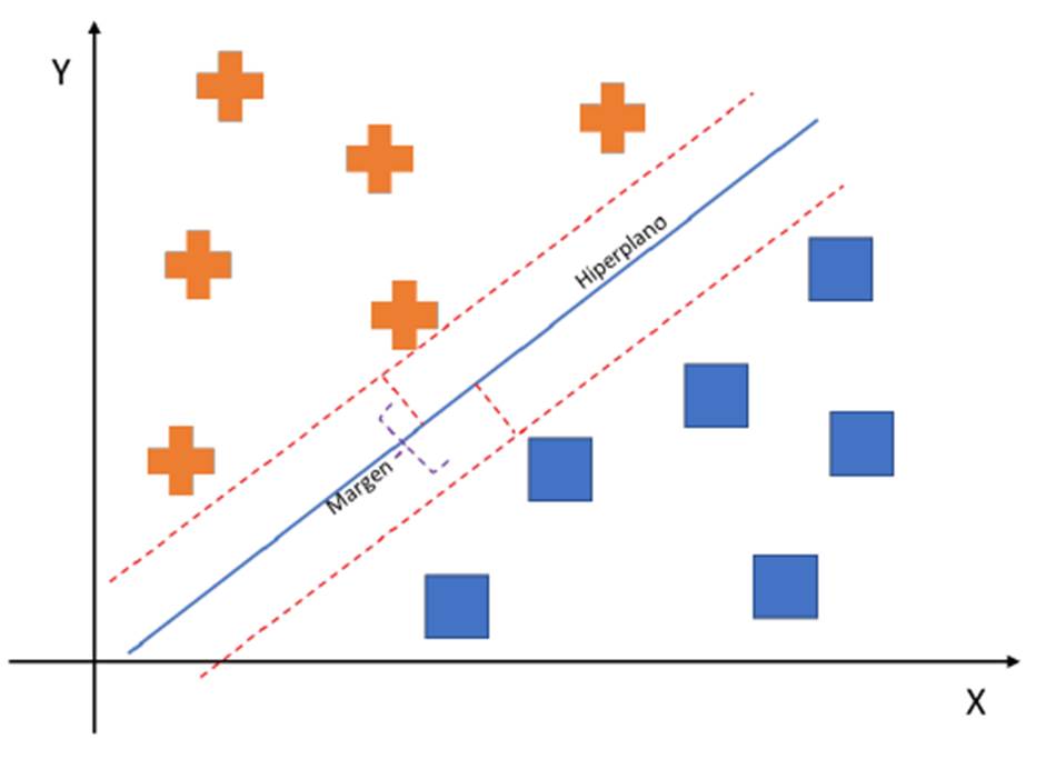
a. Support vector machine
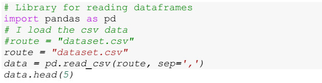
Figure 3 shows the implementation of the support vector machine (SVM) algorithm, begins with the loading of data that includes detailed information on several dengue cases, covering the period of incidence, test results, patient ages, gender, presenting symptoms, and the distinction between imported and autochthonous cases.
The panda’s library is imported into Python for the purpose of loading data from a CSV file named "dataset.csv". The specific location of that file is defined in the variable 'path', which is used as an argument in the function 'pd.read_csv()'. This function, in turn, reads the CSV file, transferring the data to a dataframe named 'data'. Subsequently, the 'head(5)' method is used to display the first 5 rows of the dataframe, allowing users to get a quick impression of the structure and content of the newly imported data.
| Period | Outcome | Age | Sex | Fever | Headache | Eye pain | Bone pain | Nausea | Rash | Imported | Autochthonous | |
|---|---|---|---|---|---|---|---|---|---|---|---|---|
| 0 | 1 | 1 | 3 | 1 | 1 | 1 | 1 | 1 | 0 | 1 | 1 | 0 |
| 1 | 1 | 0 | 1 | 1 | 1 | 1 | 1 | 0 | 1 | 0 | 0 | 1 |
| 2 | 1 | 0 | 5 | 1 | 0 | 0 | 1 | 1 | 0 | 1 | 0 | 1 |
| 3 | 1 | 0 | 5 | 0 | 1 | 0 | 0 | 0 | 0 | 0 | 1 | 0 |
| 4 | 1 | 0 | 4 | 0 | 1 | 1 | 0 | 1 | 1 | 1 | 1 | 0 |
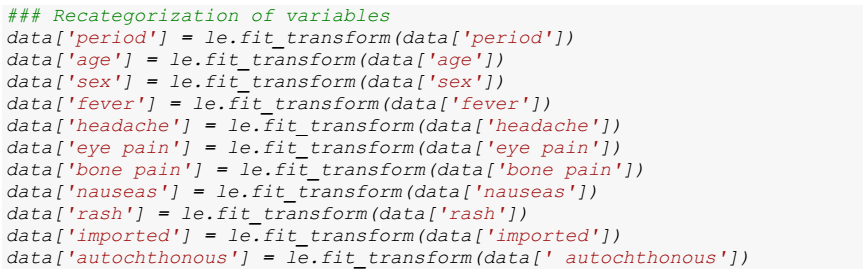
Then the transformation of categorical and binary variables to numeric variables is performed using the fit_transform method of LabelEncoder (le). This step is essential to allow the support vector machine to operate with these variables.
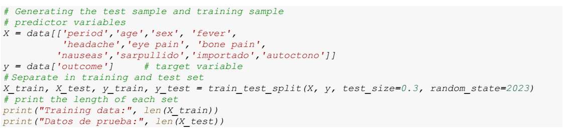
The predictor variables and the target variable for the model are defined. The set of predictor variables, denoted as X, is composed of various characteristics, such as 'period', 'age', 'sex', 'fever', 'headache', 'eyes pain', 'bone pain','nausea', 'rash', 'imported' and 'autochthonous'. These features represent the attributes that will be used to make predictions about the model output. On the other hand, the target variable, represented by Y, is associated with the 'outcome' column. This variable contains the class labels that the SVM model will seek to predict during the training and evaluation process.
Next, the splitting of the dataset into training and test sets is performed using the train_test_split function. It is important to note that 30% of the dataset is allocated for the test set, while 70% is allocated for the training set. This proportion is determined by the parameter test_size=0.3. In addition, the parameter random_state=2023 is used for the purpose of establishing a random seed and thus ensuring the reproducibility of the experiment in future runs.
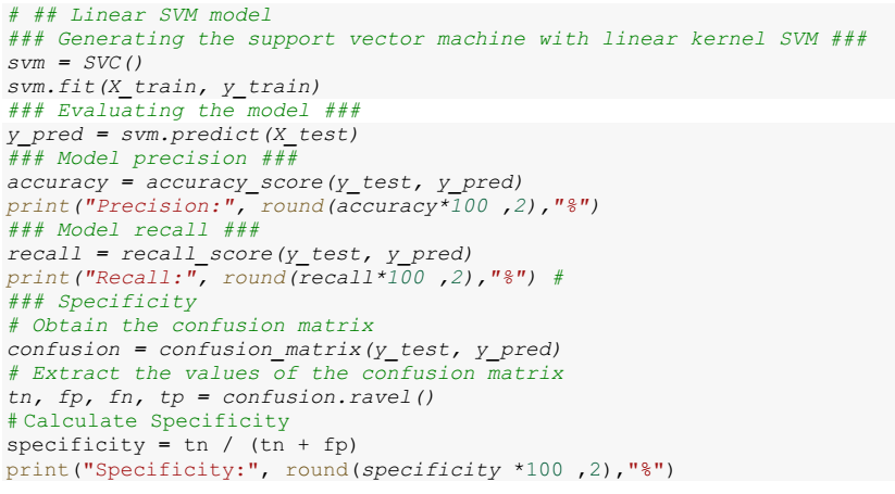
Next, an SVM with a linear kernel is created using the SVC() class. The SVM model is trained using the training set using the instruction svm.fit(X_train, y_train). The evaluation of the model is performed with the test set (X_test), where the SVM classifies the unobserved data, and the predictions are compared with the actual labels (y_test).
Various evaluation metrics, such as precision, recall and specificity, are calculated, providing detailed information on the performance of the model in terms of classification quality. (See Appendix).
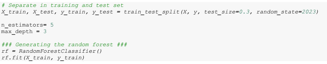
b. Random forest
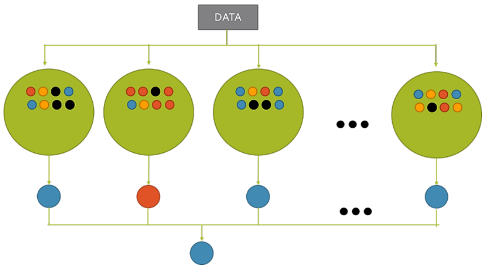
Figure 4 shows the implementation of the random forest model starts with data loading, followed by the essential transformation of categorical and binary variables to numerical variables. This step is fundamental to ensure that the random forest model can efficiently manage the variables during the training and prediction process. Next, the data set is split into training and test sets using the train_test_split function.
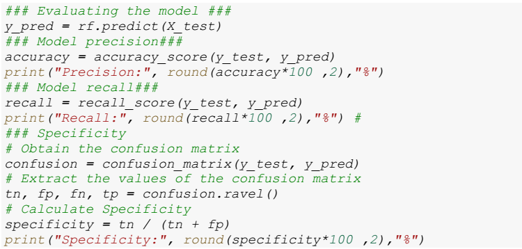
Once the preprocessing is completed, the random forest model is generated using the randomforestclassifier() class. This model is trained with the training set using the rf.fit(X_train, y_train) instruction. This step allows the model to learn patterns and relationships in the training data, preparing it to make predictions about unseen data. Model evaluation is conducted using the test set (X_test), where the random forest model classifies the unobserved data, and the predictions are compared with the actual labels (y_test). Various evaluation metrics, such as precision, recall and specificity, are calculated to provide a detailed understanding of the model performance.
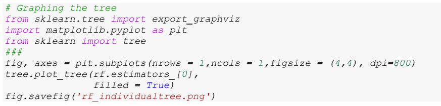
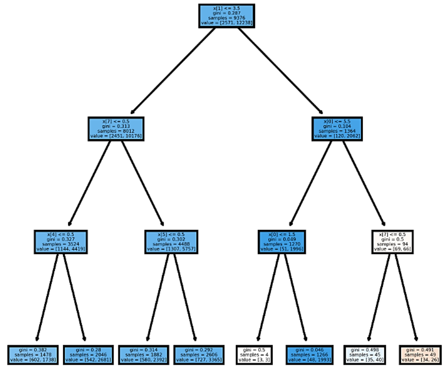
Visualizing an individual tree using tree.plot_tree (Figure 5) provides a detailed understanding of the structure and decisions made by that specific tree within the random forest. The graphical representation is saved in an image file for future analysis and reference. (See Appendix).
c. Artificial neural network
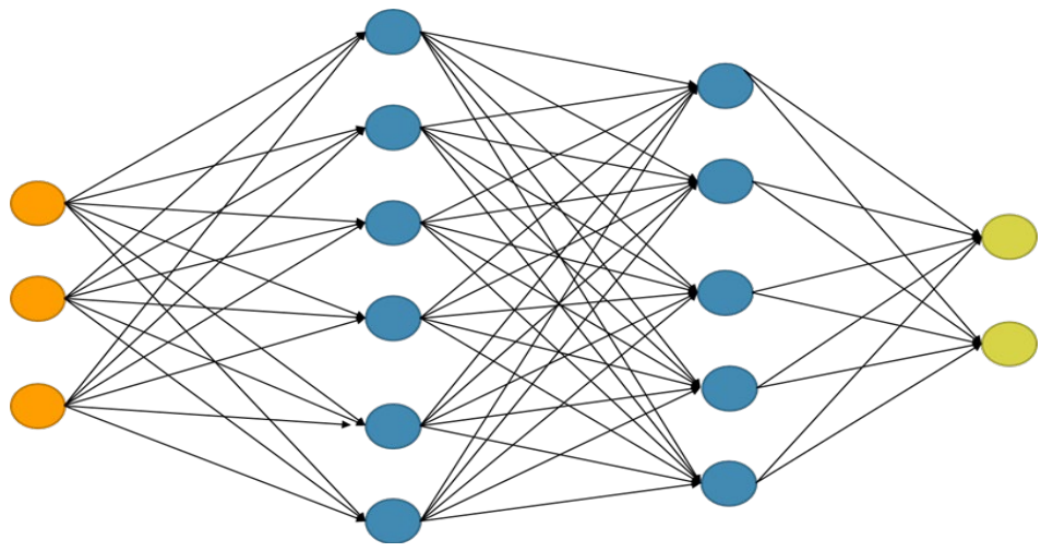
Figure 6 shows the implementation of the artificial neural network, starts with the loading of the data mentioned above. Then, the transformation of categorical and binary variables to numerical variables is performed, an essential step to allow the neural network to process and learn from these variables.
Next, the data set is split into training and test sets using the train_test_split function, ensuring an accurate evaluation of the model on data not seen during the training process.
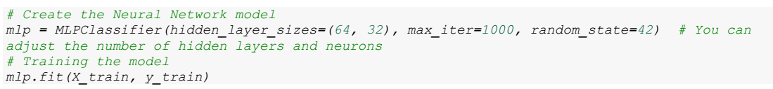
Subsequently, the Multilayer Perceptron (MLP) neural network model is built and trained using the MLPClassifier class from the scikit-learn library.
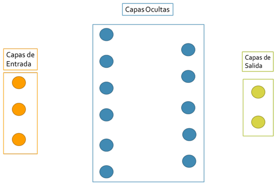
The Figure 7 shows the network architecture is specified with two hidden layers: One composed of 64 neurons and the other of 32 neurons, giving the model a certain complexity to capture patterns in the data. The model is trained with the training set using the fit method.
The evaluation of the predictive capability of the model is performed using the test set. Predictions are generated using the predict method, and evaluation metrics such as accuracy, recall and specificity are calculated. The corresponding code is presented below:
It is important to note that the ReLU activation function is employed by default in the hidden layers of the neural network. The choice of activation function is crucial, and ReLU (Rectified Linear Unit) is commonly used for its ability to manage gradient fading problems and its computational efficiency.
In addition, a maximum number of iterations (max_iter) is set for the model training process. This parameter controls the maximum number of epochs or iterations that the model will perform during training. Limiting the number of iterations can be useful to avoid overfitting and improve training efficiency. (See appendix).
2.3. Results
Table 4 presents the computational resources used by each machine learning algorithm during its execution. The support vector machine algorithm used 35.4% of the CPU, consumed 1.06 GB of RAM and exhibited a response time of 0.01 seconds. On the other hand, random forest used 21% of the CPU, consumed 1 GB of RAM and presented a response time of 0.02 seconds. Finally, artificial neural network demanded 62.3% of the CPU, used 1.32 GB of RAM and registered a response time of 0.05 seconds. (Figure 8).
Table 4 Measured CPU consumption, ram memory and response time used by the three machine learning algorithms.
| Algorithm | CPU consumption | RAM consumption | Response time |
|---|---|---|---|
| Support vector machine | 35.4% | 1.06 GB | 0.011 seg |
| Random forest | 21.0% | 1 GB | 0.024 seg |
| Artificial neural network | 62.3% | 1.32 GB | 0.051 seg |
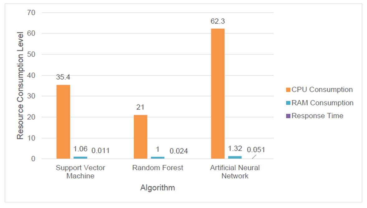
Figure 8 Measures of CPU consumption, RAM memory and response time used by the three machine learning algorithms. Own elaboration
Next, Table 5 presents the results obtained according to the performance metrics of each algorithm for dengue classification.
Table 5 Performance of the three machine learning algorithms.
| Algorithm | Precision | Recall | Specificity |
|---|---|---|---|
| Support vector machine | 83.38% | 99.05% | 8.47% |
| Random forest | 84.94% | 92.88% | 46.9% |
| Artificial neural network | 86.47% | 92.91% | 55.65% |
The results were obtained by evaluating three classification models: Support vector machine, random forest, and artificial neural network, implemented to classify dengue (Figure 9). In the first instance, the accuracy of the models was compared, revealing that artificial neural network (ANN) showed an outstanding performance with 86.47%, positioning itself as the most accurate in the classification of dengue. It is followed by the random forest algorithm with an accuracy of 84.94%, while the support vector machine presents the lowest accuracy with 83.38%.
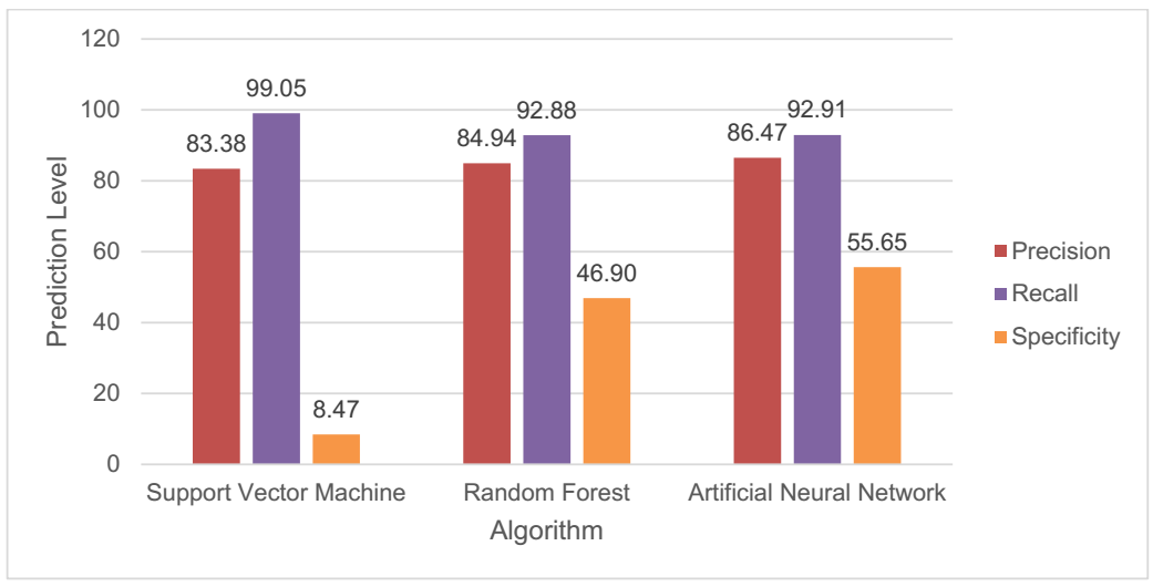
Figure 9 Performance evaluation of the machine learning algorithms proposed in our research. Own elaboration.
In the analysis of model recall, support vector machine leads with a performance of 99.05%, evidencing its ability to identify and recover a high percentage of positive cases. Random forest follows with a recall of 92.88%, and artificial neural network presents the lowest recall with 92.91%.
Finally, the comparison of the specificity of the models shows that artificial neural network exhibits the best performance with 55.65%, indicating its ability to correctly identify and classify a high percentage of negative cases in relation to the total number of negative cases. Random forest obtains a specificity of 46.9%, while support vector machine presents the lowest specificity with 8.47%.
2.4. Discussion
The results obtained in this study, focused on a comparative analysis of machine learning algorithms for dengue classification, offer valuable insights that contribute to the advancement of diagnostic tools in clinical practice. The application of various machine learning algorithms has yielded encouraging results in terms of accuracy and recall in dengue classification.
The analysis revealed that the support vector machine algorithm demonstrated a sensitivity of 99.05%, outperforming other approaches. This feature facilitates resource optimization by identifying the most efficient algorithms, contributes to the identification of features and risk factors associated with dengue, and supports clinical decision making, while contributing to scientific progress in the field of medicine.
However, it is crucial to address the limitations identified during the study. The dataset has limitations in the generality of symptom information, the binary categorization of outcomes that simplifies clinical complexity, and the age grouping that may not capture intragroup variability. The autochthonous/imported distinction could be more specific, and the monthly categorization may lack sufficient temporal detail. Data quality and consistency, biases, and ethical considerations are issues to be addressed to improve the reliability and usefulness of the dataset.
Comparing the results with previous research, it is noted that Mello-Roman et al. reported a recall of 93% for the support vector machine algorithm, which is lower than the figure obtained in our research. In their study, they used a dataset of real patients with a previous diagnosis of dengue fever, extracted from the Paraguayan public health system. Ozer et al. reported that the support vector machine algorithm had a recall of 76%. In their study, they used SISA and SISAL datasets that include demographic information, past medical histories, and symptom data.
The practical implications derived from the results indicate that the implementation of machine learning algorithms has the potential to significantly improve dengue classification. However, the transition from the research setting to clinical application poses additional challenges, such as integration with existing medical information systems and validation of results in real-world clinical settings.
This analysis provides significant insights into the efficiency of machine learning algorithms in dengue classification, highlighting the importance of future research that addresses specific challenges or supports the clinical application of these promising tools.
3. Conclusions
This comparative study of machine learning algorithms for dengue classification has provided valuable insights into the performance and effectiveness of different methodologies. The results highlight the significant potential of these tools in improving diagnostics and efficient identification of dengue cases. The main findings are presented below: Support vector machine (SVM) performance: The SVM algorithm proved to be sensitive, reaching a sensitivity of 99.05%. This ability to accurately identify positive cases highlights the effectiveness of SVM in the classification of dengue cases. Despite encouraging results, limitations are recognized in the generality of symptom information, binary categorization of results, and age grouping. These should be addressed in future research to improve the quality and utility of the data set. Comparison with previous studies reveals variations in results, highlighting the importance of considering the particularities of each data set and context. Variability in results highlights the need for additional studies to validate and generalize findings.