


 nueva página del texto (beta)
 Inglés (pdf)
 Artículo en XML
 Referencias del artículo
 Enviar artículo por email
 Citado por SciELO
  Similares en
SciELO
Similares en
SciELO 
 Permalink
1. Introduction
Brain-computer interface (BCI) systems operate under conditions of real-time interactions and response immediacy, demanding electrophysiological signals to be acquired and processed with low latency for effective communication between processing computers and elicited brain activity. BCI devices are often used to obtain encoded signals containing user intention of movement execution through the motor imagery (MI) paradigm, which has proven to be more effective at engaging cortical motor areas and related networks to a significant extent. Virtual reality, neurorehabilitation, and robotic device control are just a few of the many uses for MI BCI systems. However, online BCI systems, such as MI-based control systems for exoskeletons, may need to translate brain signals quickly and precisely into physical actions (Choi et al., 2020; Cho et al., 2021). In this regard, latency, which becomes a deterministic factor in these systems' effectiveness, is influenced by the system’s hardware, software, and firmware, as seen in research utilizing platforms such as BCI2000 and g.USBamp. As a result, MI BCI systems are subject to variations in latency that impact user-computer interactions (Schalk et al., 2004; Wilson et al., 2010).
On the other hand, offline BCI systems are also widely used to conduct post-hoc brain signal analysis, allowing more computationally intensive algorithms to train and improve classification models. These systems are essential for the research and development of new classification and feature extraction techniques, such as deep learning (DL) and more advanced feature extraction to improve the decoding of neural activity (An et al., 2014; Echtioui et al., 2021; Schirrmeister et al., 2017). Yet, the need for a balance between computational efficiency and precision is highlighted by the fact that while these methods improve precision, they also raise the costs and computational power required (Changoluisa et al., 2020; Netzer et al., 2020).
Consequently, specific BCI frameworks for integrating EEGNet and other deep learning algorithms are pushing innovation in EEG signal classification and feature extraction. Moreover, including metrics for neural networks in BCI control systems for robotics has proven to be a promising area of research. Overall, the adoption of these algorithms devoted to MI-BCIs systems has allowed more precise decoding of a subject’s thoughts, with studies like NeuroGrasp, which integrate EEG and EMG signals for the classification of different kinds of hand grips (Cho et al., 2021). However, the implementation of these techniques in real-time still needs to be improved due to the time required to train these deep learning models.
This work develops a real-time feedback mechanism for a BCI by analyzing EEG data using a deep learning model. Experiments conducted on a real-world application task demonstrate that the low-cost and portable design of the system enables the MI paradigm to function well in situations with poorly controlled sampling.
2. Materials and methods
2.1. Architecture of BCI-based system for EEG Analysis
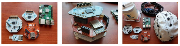
Data Acquisition System: This Python module, integrated within SDK vendors, enables data acquisition using OpenBCI Cyton boards with driver compatibility. These versatile boards support multiple modes of electrode interconnection, including monopolar, bipolar, and sequential, making them suitable for a wide range of research and development applications. The flexibility in electrode configuration allows researchers to tailor the setup according to specific experimental needs. Additionally, the system’s capacity to expand up to 16 monopolar channels provides greater flexibility in data sensing, accommodating complex experiments that require extensive monitoring.
The acquisition system not only captures data efficiently but also seamlessly integrates an acquisition interface within the overall framework. This interface facilitates real-time data visualization and immediate feedback, enhancing the user experience during data collection. The integration supports the creation of a comprehensive database that stores all relevant metadata, including subject information, experimental conditions, and sensor configurations. Automatically synchronized markers ensure precise alignment of events and recorded signals, which is crucial for accurate data analysis. Furthermore, the system is designed to be robust and scalable, capable of handling large datasets and adapting to increasing data acquisition demands. This robustness ensures reliability and consistency across various experimental setups and conditions.
Communication module: The module for conveying information is mainly built on Apache Kafka, serving as the backbone for supporting a distributed communication system across the entire architecture. Even though analyzing EEG neural responses requires fast and reliable data transmission, this module also supports slow communication via WebSockets. Thus, using a Wi-Fi shield, the maximum sample rate can be increased from 250 Hz to 16 kHz for eight channels. Simple read-and-write commands perform communication between the computer and the board. Also, the module supports Message Queue Telemetry Transport (MQTT) and TCP, with TCP being the preferred choice due to its simplicity. As regards OpenBCI, it is based on ADS1299, a 24-bit analog-to-digital converter from Texas Instruments. In addition to offering flexibility in sampling rate, number of channels, and protocols, the communication module ensures that EEG data blocks will be ready within a time less than their duration.
Distributed module for stimuli delivery: The module delivers elicited stimuli through a remote presentation system based on a conventional web application developed using HTML, CSS, and the JavaScript Brython-Radiant framework. This web-based approach ensures compatibility across different devices and platforms, facilitating widespread accessibility and ease of use. Additionally, integrated development environments (IDEs) provide easy-to-use APIs for creating custom visualizations, allowing researchers to tailor the presentation of stimuli to specific experimental requirements. These APIs enable the development of sophisticated visual stimuli with minimal coding effort, enhancing the flexibility and functionality of the system. The main interface of the module incorporates a mechanism for calculating and correcting latency during stimulus delivery. This latency correction mechanism is crucial for ensuring precise timing and synchronization of stimuli, which is essential for experiments that require exact temporal control. The system continuously monitors latency and applies real-time corrections to maintain accuracy. Furthermore, the interface allows for detailed logging and analysis of stimulus presentation data, providing researchers with comprehensive insights into the timing and effectiveness of their stimuli. This robust and scalable design ensures reliable performance across various experimental conditions and setups, making the module a valuable tool for researchers in diverse fields.
Real-time EEG-NET BCI processor: The EEG-NET Data Processing Block within the BCI framework is a pivotal element for real-time EEG data analysis and closed-loop BCI applications. Utilizing a convolutional neural network (CNN) architecture optimized explicitly for EEG signals, this block is implemented in Python and leverages machine learning frameworks like TensorFlow or PyTorch. It integrates with the existing Data Acquisition System and Communication Module, receiving raw or preprocessed EEG data via Apache Kafka streams. The real-time processing capabilities of this block enable immediate feedback, thereby closing the loop in BCI applications. This property facilitates various real-time neurophysiological interventions, from neurofeedback to adaptive BCI systems. This module can be tailored to meet the needs of a broad class of experimental setups thanks to its modularity and flexibility in configuration.
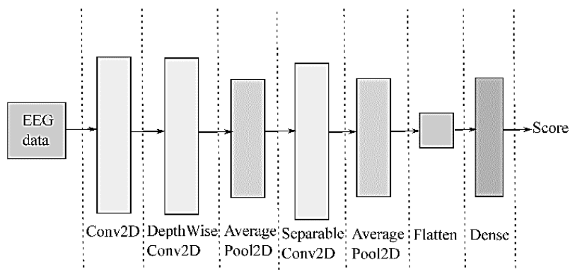
Deep Learning-based EEGnet framework: For supporting EEG analysis with deep learners, the compact EEGNet convolutional network provides convolutional kernel connectivity between acquired neural responses and extracted feature maps, enabling its use in different MI paradigms. Figure 2 shows that the EEGNet pipeline initiates with a temporal convolution to learn frequency filters, followed by a depth-wise convolution connected to each feature map. As a result, frequency-specific spatial filters can be learned. Further, the separable convolution combines a depth-wise convolution, which infers a temporal summary for each feature map individually, followed by a point-wise convolution, which identifies how to mix the feature maps optimally for class-membership prediction.
2.2. Data Acquisition of EEG neural responses. The following procedures are developed for the acquisition of neural activity:
Electrode deployment over the scalp:
At the beginning of the data acquisition procedure, the subject’s hair must be washed with salt-free shampoo or coconut soap to cleanse it thoroughly. Then, the hair must be adequately dried with a towel and a hairdryer adjusted to room temperature.
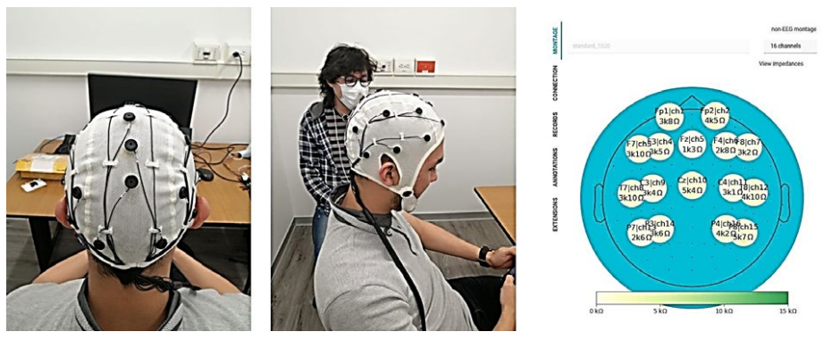
The cap is positioned on the subject so the reference electrode CZ is at the center of the head (The operating EEG montage is 10-20). The ears and nose, seen from above, are used as references, as shown in Figure 3.
Once the cap is correctly positioned on the subject’s head, the "Electro-gel" substance is applied with a syringe to ensure an adequate amount between the electrode and the scalp. It is worth noting that care must be taken to ensure that the gel from one electrode does not mix with that of another, as this can affect measurements of electrical signals on the scalp.
The acquisition of elicited EEG neural activity can be performed after completion of the electrode placement and impedance calibration (this procedure is described below). Finally, use a brush and alcohol or a cotton swab to remove excess gel from the electrodes on the cap and allow it to dry. Impedance Calibration of Electrode-Montages: The impedance measurement is performed by simultaneously feeding a 6 nA alternate current at 31.2 Hz to the whole electrode arrangement. The activated electrodes are set up in the correct mode following the lead-off-impedance method (Cardona Álvarez, 2022).
After ensuring the Cyton board is correctly plugged in, a 10K potentiometer is connected between the N input (bottom) of channel one (1) and the SRB2 device (bottom). Note that this pin must be turned on if calibration is performed directly on the head instead of a potentiometer. Otherwise, the BIAS pin will not be used.
Further, the actual value of the impedance Z is computed as follows:
Where
Since the Cyton board holds a 2.2 kOhm resistor connected in series with each electrode, this value must be removed to avoid biased measurements of the Z impedance. Then, after the electrode-subject impedance is emptied, the impedance range of 1-10 kOhm is set to ensure the amplitude of either recording activity, EEG or EOG, does not change during measurements (Shad et al., 2020).
The above-described impedance calibration is automated over the entire EEG montage using the interface displayed in Figure 3, coloring in green those electrodes with impedance values within the proper range. In contrast, the wrong electrodes are colored in red. In the latter case, the cap should be adjusted or more gel applied, ensuring no contact between the electrodes during measurement.
3. Experimental set-up
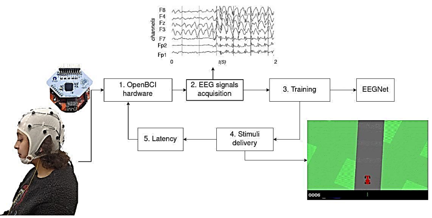
As illustrated in Figure 4, we assess the developed BCI-based Real-Time system for Implementing Deep Learning Frameworks for a specific instance of the MI paradigm. The system evaluation comprises the following stages: i) Database collection of four classes of MI data, ii) Testing on real-time processing of the BCI system for classification of MI tasks.
Database collection of 4-Class MI neural responses
The system was configured for 16 channels, with a sampling rate of 1000 samples per second per channel, with a monopolar montage following the standard 10-20 montage. The data was acquired on ten subjects performing four MI tasks (left-hand, right-hand, foot, and tongue). Each subject would perform these tasks upon an arrow appearing onscreen (up arrow for the tongue, left side arrow for the left hand, right side arrow for the right hand, and down arrow for the feet), with an asynchronous pause (between 2000 and 3000 ms) between each cue, as adjusted in Cho et al. (2017).
3.1. Preprocessing stage
The preprocessing step is as follows (Lawhern et al., 2018):
We load subject recordings using a custom database loader module: https://github.com/UN-GCPDS/python-gcpds.databases. The trial is set to a zero-amplitude signal upon a system failure during the acquisition (note that these trials are discarded at this stage). Next, each properly acquired signal is downsampled from 512 Hz to 128 Hz using the Fourier method provided by the SciPy signal resample function: https://docs.scipy.org/doc/scipy/reference/generated/scipy.signal.resample.html. Then, each time series trial is filtered between [4, 40] Hz, using a fifth-order Butterworth bandpass filter. In addition, we clip the records within the range of [0.5 - 2.5] s after the stimulus onset for the GigaScience database and from 2.5 s to 4.5 s for the BCI-Framework-Unal database, retaining only the information corresponding to the MI task. Since only the MI time segment will be considered, we assume just the signal stationarity within this interval.
With this straightforward preprocess, we aim to investigate five distinct brain rhythms within the 4 to 40 Hz range: theta, alpha, and three beta waves. Theta waves (4-8 Hz), located in the hippocampus and various cortical structures, are believed to indicate an "online state" and are associated with sensorimotor and mnemonic functions (Abhang et al., 2016). In contrast, sensory stimulation and movements suppress alpha-band activity (8-13 Hz), modulated by attention, working memory, and mental tasks, potentially acting as a marker for higher motor control functions. This range also comprises three types of beta waves: low beta waves (12-15 Hz), or "beta one" waves, mainly associated with focused and introverted concentration; mid-range beta waves (15-20 Hz), or "beta two" waves, linked to increased energy, anxiety, and performance; and high beta waves (18-40 Hz), or "beta three" waves, associated with significant stress, anxiety, paranoia, high energy, and high arousal.
4. Results
4.1. Real-time classification of MI tasks
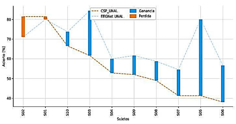
The comparative analysis in Figure 5 between CSP (Cho et al., 2017) and EEGNet (Lawhern et al., 2018) methods for EEG signal classification has indicated a substantial average increase of 21.6% in accuracy for EEGNet, with CSP yielding an accuracy of 56.54% ± 8.78 and EEGNet 68.09% ± 10.73. Nonetheless, the study by Tobón-Henao et al. (2022) suggests a decrease in accuracy for some subjects, which may be attributed to a generalized signal-to-noise ratio reduction approach that does not account for individual signal quality, negatively impacting those with superior EEG signals. This issue results in a tailored application of noise reduction techniques to preserve the integrity of high-quality EEG signals across subjects.
Training and measured latency. An EEGNet model is trained to classify EEG signals in real-time for inputting commands using MI. In the test environment, the subject controls a video game car from Car-Racing (https://www.gymlibrary.dev/environments/box2d/car_racing/). The car constantly moves forward, and the user must steer left or right to stay on the track. The acquisition, preprocessing, and training are all done in real-time.
Given that the model requires a time window of 2500 ms, corresponding to the MI window, the system was configured to classify the user’s EEG every 500 ms. Latency is the time between acquiring the last 100 ms packet and the classification. This latency includes everything from deserialization, transmission, and reading carried out by the BCI-Framework to the time it takes for the model to classify the signals successfully.
In order to measure latency, we used the predictor from the trained EEGNet model. This model was trained using an MI test with a stimulus duration of 3000 ms and an asynchronous stimulus onset ranging from 1000 to 1500 ms; the MI duration was trimmed to 2500 ms. For the validation test, a stimulus of 10000 ms with an asynchronous onset of 3000 ms was used, ensuring that the same subject, protocol, and paradigm were applied in different sessions and on different days. In Figure 6a, it is observable that some latencies exceed 20 seconds, which is attributable to transmission errors and a no-packet-loss policy. Figure 6b displays the expected latencies with a value of 150 ms from the fourth data block processed and a jitter affected by 100 ms packetization used during transmission.
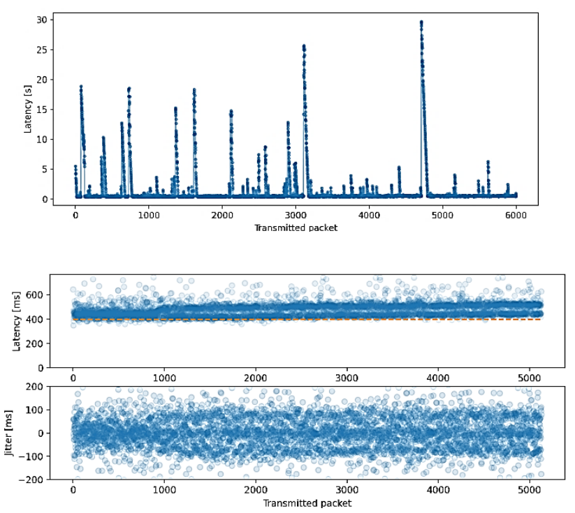
Figure 6 Measurement of latencies and their deviation: (upper) Latency for 6000 consecutive packets, (lower) The standard deviation (jitter) remains within a range of about 150 ms.
According to the BCI-Framework, the expected latency should be 456 ms, corresponding to the first four 100 ms packets and the preprocessing of the entire window. As seen in Figure 6a, the latency sometimes exceeds the expected value of 456 ms. This result is due to the intermittencies between packets and TCP’s no data loss policy. However, in Figure 6b, we can see how, ultimately, the latencies cluster around this expected value.
Offline inference over sliding windows. To examine the model’s behavior on a constant flow of data, as shown in Figure 7a, an experiment was conducted in which MI data was compiled over ten seconds, preceded by three seconds of non-MI activity. This setup was chosen to simulate a more realistic scenario where the model needs to distinguish between periods of activity and inactivity. It is worth noting that the reference point (t=0) is located at the start of the MI task segment, providing a clear demarcation for evaluating the model’s performance. This reference point serves as a crucial marker, enabling a precise analysis of how the model transitions from non-MI to MI data and its subsequent impact on prediction accuracy. The experiment consisted of shifting a 2s-window every ten samples. This approach allowed for a detailed assessment of the model’s temporal dynamics and its ability to adapt to changing data patterns. The blue line in the graph represents the model’s average confidence (as a supervised task) in making correct predictions, providing a quantitative measure of its reliability over time. The shaded area around the blue line indicates the standard deviation, offering insights into the variability and consistency of the model’s predictions.
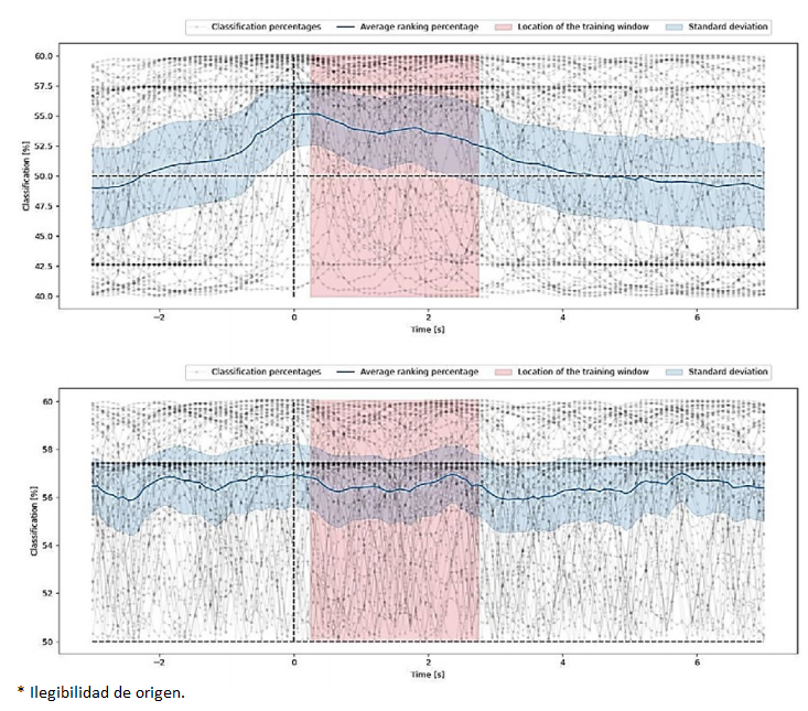
Figure 7 Real-time classification analysis using sliding windows, depicting individual classification percentages, moving average, and standard deviation, highlighting the model’s training period: (upper) Sliding Window Classification, (lower) Unsupervised Sliding Window Classification.
The accuracy of the model increases as the sliding window reaches the MI segment, reaching its peak when it overlaps the same time segment used to train the model (shown in pink). This peak accuracy indicates the model’s ability to generalize well from training data to real-world scenarios. Figure 7a represents the accuracy for the supervised task, whereas Figure 7b delivers the accuracy for the unsupervised task, highlighting the differences in model performance under varying conditions.
From the previous findings, we hypothesize that the validation threshold can be adequately fixed to generate control signals for a given application by measuring the model’s accuracy and placing the reference point at the end of the MI segment, just like an actual prediction environment. This hypothesis suggests that by fine-tuning the validation threshold, it is possible to enhance the model’s practical utility in real-time applications. Placing the reference point at the end of the MI segment simulates a real prediction environment where timely and accurate control signals are crucial. This approach not only improves the model’s performance but also ensures that the generated control signals are reliable and can be effectively used in various applications, such as BCIs or other neurotechnological systems.
5. Conclusions
For illustration purposes, some BCI real-time systems for AI are shown in Figure 1 and detailed in Table 1. Most of these systems do not share information about latency or how to measure it, and they all have different sample frequency and channel settings (see Table 1 for system configurations).
Table 1 Different configurations of BCI systems that utilise artificial intelligence and are deployed in real time.
| BCI System | Fs | Channels | Latency |
|---|---|---|---|
| Hybrid BCI + actiCHamp (Choi et al., 2020) | 500 Hz | 31 | ±1020 ms |
| NeuroGrasp + BrainAmp (Cho et al., 2021) | 1000 Hz | 20 | - |
| BCI-reinforcement learning + g.USBamp (Pires et al., 2022) | 256 Hz | 16 | - |
| Functional Brain network + UE-16B (Ai et al., 2019) | 1000 Hz | 16 | - |
| BCI-Framework EEGNet (Ours) | 1000 Hz | 16 | ±150 ms |
High latency issues are critical in real-time data processing as they can severely disrupt the timeliness and reliability of system responses. In BCIs, where immediate feedback is essential, elevated latencies may lead to mismatches between user intention and system action, undermining the effectiveness and user experience of handling BCI devices. Therefore, minimizing latency is imperative to maintain the seamless integration of such systems with user activities, ensuring their practical applicability and user acceptance.
The capability to implement our system in real-time and close the feedback loop stands as a significant advantage. It allows instant interaction between the user and system, facilitating a more intuitive and efficient BCI experience. This immediacy is paramount, particularly in applications requiring rapid decision-making, as it ensures that the system can keep pace with the user’s cognitive processes, resulting in a harmonious and effective integration of technology and human intent.
Overall, we present a low-cost, portable system for EEG-based BCI-MI real-time applications. We performed all the stages of a closed-loop system, from the data acquisition to the inference of commands utilizing Machine Learning, while also handling latency for validation.
Our low-cost EEG database presents competitive results compared to publicly available datasets.
Regarding offline training on the GIGAScience and the BCI-Framework Unal databases under our approach, its capacity for more precise discrimination of MI data becomes evident compared to traditional techniques such as CSP. This improvement is clearer for individuals with poor to moderate MI skills.
Online training shows how our model can run in real-time settings, guaranteeing a proper response in an opportune manner for the user.
Offline classification with sliding windows showed promising results, considering the variability from the experiment being conducted in a different session.

