1. Introduction

The mechatronic device known as the Furuta pendulum was devised by ^{Furuta and colleagues in 1991}-their findings were first reported in the paper by ^{Furuta et al. (1991)}. In this paper, Furuta and colleagues brought attention to their novel pendulum, showing its usefulness for education in control engineering. Since then, the Furuta pendulum has become a popular expression, representing a pendulum with two rotary arms, as depicted in Figure 1.

Figure 1 The Furuta pendulum with its coordinate system. 

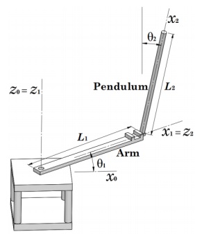
As can be seen in Figure 1, the Furuta pendulum mechanism has two degrees of freedom. Indeed, the mechanism contains three main parts: base, horizontal arm, and vertical arm (i.e., pendulum). The base hosts a direct-current (DC) motor that produces rotational movement in the arm. On one of its sides, the horizontal arm remains attached to the motor's rod. On the other side, the horizontal arm is attached to the vertical arm, which in turn produces the pendulum movement, see ^{Furuta et al. (1991)}, ^{Zabihifar et al. (2020)}, ^{Hazem et al. (2020)} for further details on the construction of the Furuta pendulum. The Furuta pendulum has been studied not only in control education (^{Galan et al., 2019}; ^{Alves et al., 2022}), but also in applications such as aerospace (^{Shoyama et al., 2021}), robotics (^{Hofer & D’Andrea, 2018}), and underwater vehicles (^{Duecker et al., 2018}).

Motivated by the fact that the Furuta pendulum is nonlinear, unstable, and underactuated, researchers have become interested in developing different strategies to control and stabilize its mechanism. Plenty of studies have documented control for the Furuta pendulum. For instance, a study has proposed the so-called active disturbance rejection control to diminish undesirable effects of nonlinearities in the system response (^{Ramírez- Neria et al., 2014}).

Another study has introduced a control based on feedback linearization, which is taken from the position and velocity error functions (^{Aguilar-Avelar & Moreno-Valenzuela, 2015}). In ^{Moreno-Valenzuela et al. (2016)}, the authors have presented an adaptive neural network control, showing numerical evaluations for PID with neural networks. The authors of ^{Cruz et al. (2017)} show an exhaustive procedure that determines the controller gains through all possible gain combinations, picking the controller that generates the best system response. The study of ^{Pujol-Vazquez et al. (2018)} presents a magnetic device that allows the arm of the Furuta pendulum to work with H∞ control. In ^{Zhang and Dixon (2021)}, a non-minimum state feedback controller is presented with the anti-windup integrator to stabilize the Furuta pendulum. A recent study shows the control of the Furuta pendulum via a sliding mode control (SCM), illustrating the benefits of SMC for decreasing vibrations in the underlying mechanism (^{Nguyen et al., 2020}). In ^{Dwivedi et al. (2017)}, the fractional order PID controller is developed using a control parameter adjustment technique through gain margin, phase margin, and Nyquist graph; the application of this technique improves the robustness of the controller. The approach of ^{Yang and Zheng (2018)} shows trajectory planning so that the pendulum oscillates from its downright position to its upright position; this task is accomplished through the adaptive neural network with linear matrix inequalities. What the research from these papers taken together suggests is that the control of the Furuta pendulum remains a challenge.

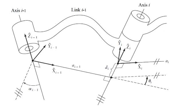
The main contribution of this paper is to show simulation data from a virtual prototype Furuta pendulum. This prototype worked with the classical linear quadratic regulator with integral action (LQR+I) control during the simulations. To adjust the LQR+I parameters, we use the pendulum's model, as usual in the literature (^{Ramírez- Neria et al., 2014}). Note that the pendulum's model can be obtained from both the Euler-Lagrange formulation ^{Cazzolato and Prime (2011)}, ^{Fantoni and Lozano (2002)} and Kane's method ^{Hamza et al. (2019)} -the dynamics from both methods coincide. Even though the Euler-Lagrange formulation has been covered in the literature ^{Cazzolato and Prime (2011)}, ^{Fantoni and Lozano (2002)}, we decided to revisit it here using virtual prototyping to reliably validate the mathematical modeling of a complex system, in this case, the Furuta pendulum. Where it is possible to identify whether the simplifications in the model don’t differ too much from the model created through virtual prototyping that doesn’t have these simplifications and consumes less time to be made. And suggest a reference (^{Moura, 2021}) on which this paper is based that presents the development of mathematical modeling using the Euler-Lagrange method, explaining a greater number of steps and considerations regarding them that facilitate the understanding of the application of the methodology. Another important point was that the coordinate system that referenced the links was positioned using Denavit-Hartenberg's parameters, as in the coordinate systems that reference the links, the z-axis is positioned according to the degree of freedom of the joint and the x according to the length of the link which makes it easier to know where the parameters αi-1, ai-1, di e θi are as shown in Figure 2.

Figure 2 Connection of two subsequent links according to Denavit-Hartenberg (^{Craig, 2005}). 

An interesting conclusion from our simulated data is that the LQR+I control seems to stabilize the Furuta pendulum. Namely, we simulate the Furuta pendulum in two distinct ways: (i) nonlinear dynamics from the Euler-Lagrange formulation and (ii) virtual prototyping designed in the Adams software (Newport Beach, California, USA). The simulated data from both models suggest that the Furuta pendulum is stable under the LQR+I control. This numerical evidence emphasizes the potential of the LQR+I control for stabilizing the Furuta pendulum.

Remark 1: To the best of the authors' knowledge, there is no proof that the LQR+I control stabilizes the Euler-Lagrange model representing the Furuta pendulum. No formal proof is available.

Our conclusion that the LQR+I control seems to stabilize the Furuta pendulum only comes from observing simulated data. Yet it is worth emphasizing that no definitive conclusion about stability can be drawn only from simulated data.

This paper is organized as follows. Section 2 presents the Euler-Lagrange modeling of the Furuta pendulum and its main parameters. Section 3 shows the linear control strategy and the corresponding simulated data. Finally, Section 4 presents some concluding remarks.

Notation: The symbol Rn denotes the nth dimensional Euclidean space. The superscript T on UT denotes the transpose when U represents either a vector or matrix. The operator diag(a1, ... , an) defines the diagonal matrix of dimension Rn×n comprising the elements a1, ... , an arranged in its main diagonal. We borrow from ^{Cazzolato and Prime (2011)} the notation that defines the dynamics of the Furuta pendulum.

2. Dynamics of the Furuta pendulum

Recall that the ‘control goal’ of the Furuta pendulum is to balance its pendulum in the inverted position through torque control. The torque must be applied to keep the angle θ2 as close as possible to zero, i.e., driving the arm L2 to the vertical position (see Figure 1). To generate this torque, we rely on a DC motor that rotates the arm L1 around the axis Z0, thus generating the angle θ1. While increasing or decreasing θ1, the DC motor keeps applying torque τ1 upon the arm L1. The arm L2 moves freely because its joint with L1 has no actuator. As in ^{Cazzolato and Prime (2011)}, we assume that m1 and m2, located at l1 and l2, represent the mass of the two arms. The two arms are damped by the constants b1 and b2.

Next, we present the Euler-Lagrange formulation that represents the dynamics of the Furuta pendulum.

2.1. Euler-Lagrange formulation: Nonlinear dynamics for the Furuta pendulum

Next, we use the notation borrowed from ^{Craig (2005)} [Ch. 2 and 6] to represent the system of coordinates of the Furuta pendulum.

Let us denote the fixed coordinate system by {0}. As indicated in Figure 1, the coordinate systems are {0}, {1} and {2}, and they correspond to (x0, y0, z0), (x1, y1, z1), and (x2, y2, z2), respectively. The coordinate system{0} shows the initial position of the arm. The coordinate system {1} shows the displacement performed on the arm. The coordinate system {2} shows the pendulum's observed displacement due to the arm's displacement. More details are given below.

The coordinate system {1} moves with the arm. To the displacement of the arm, the z-axis {0} is rotated for θ1. To describe the pendulum's displacement, the y-axis is rotated in -π/2 radians and moved L1 along the x-axis. The x-axis is then rotated in π radians. Finally, the z-axis is rotated in θ2. The coordinate system {2} moves with the pendulum itself.

Using Euler angles, we can write the rotation matrices R of the arm as (^{Craig, 2005,} Ch. 2):

and of the pendulum as:

Following the notation of ^{Cazzolato and Prime (2011)}, we denote the axial moment of inertia in the x-axis by I1x for the arm and by I2x for the pendulum and, respectively, by I1y, I1z, I2y, I2z for the other corresponding axes (the unity of moment of inertia is kg.m2).

Define the function F1 : R6 → R as:

and F2 : R6 → R as:

Now, we can present the main result of this section. The nonlinear dynamics of the Furuta pendulum are given by:

The pendulum rotates freely. Then there is no external torque applied to it. Thus, τ2= 0. That proves the underactuated system, with 2 DOF (rotation in the arm and rotation in the pendulum) and only one torque applied (τ1 in the arm).

2.3. Virtual prototyping of the Furuta pendulum

A prototype of the Furuta pendulum was developed in SolidWorks (Waltham, Massachusetts, USA), see Figure 3.

Figure 3 Furuta pendulum prototype developed in SolidWorks. 

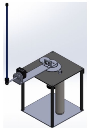
The prototype features were extracted from SolidWorks, see Table 1. These features were later transferred to the virtual prototyping software Adams (Newport Beach, California, USA) because Adams can emulate the real-time dynamics of a Furuta pendulum.

3. Linear state-feedback control: Numerical evaluations

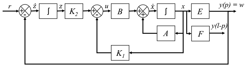
We have two nonlinear models. The first was obtained by analytical calculation, and the second by virtual prototyping. For the LQR application, it is necessary to calculate the linear format of the two models. Just after, it is possible to calculate the LQR gains. The LQR provides a multivariable proportional regulator, where it is necessary to add an integrator to the controller to eliminate steady-state errors between the reference signal and the controlled state variable, which in this case is the angular position of link 1. Therefore, the LQR control needs to have integral action. The block diagram of one LQR with the integral action, also known as LQR+I, is shown in Figure 4.

Figure 4 Block diagram for the LQR+I control (adapted from ^{d’Azzo & Houpis, 1995}). 

Then, we linearized the model obtained with the Euler-Lagrange formulation and configured the computational calculation to result in the linear model. Thus, we found the gains K1 and K2 with the linear models for both cases.

The matrices in (9) and (10) corresponding to the features in Table 1 are:

By virtual prototyping, the matrices are:

It is important to emphasize that the most significant values are in different positions in the two models because the states' position in the state vector differs between them.

Next, we revisit the tracking control of linear systems (^{Ostertag, 2011}, Sec. 1.8). For a given reference signal r ∈ R, we compute the error signal, i.e., e = r - y ∈ R where y=10   ⋯0x, and x ∈ R4 satisfies (7) - (10). Define zt≡∫0teτdτ for all t ≥ 0, and:

Since z˙=e we can write (^{Ostertag, 2011}, Sect. 1.8.1):

The control problem consists of finding the gains K1T∈R4 and K2∈R that minimizes the linear-quadratic-regulator with the integral action (LQR+I) cost with r≡0 (^{Anderson & Moore, 1989}, Ch. 3; ^{Rosinová & Veselý, 2006}, p. 196):

It is known that the minimum value of (15) is attained when solving the usual Riccati equation (^{Anderson & Moore, 1989}, Ch. 3). In our case, the optimal solution for the model given by (11) is:

and for the model given by (12) is:

provided that Q = diag(0.001,  0.01,  10-4, 10-4) and R = 15. The values of Q and R were chosen by trial and error.

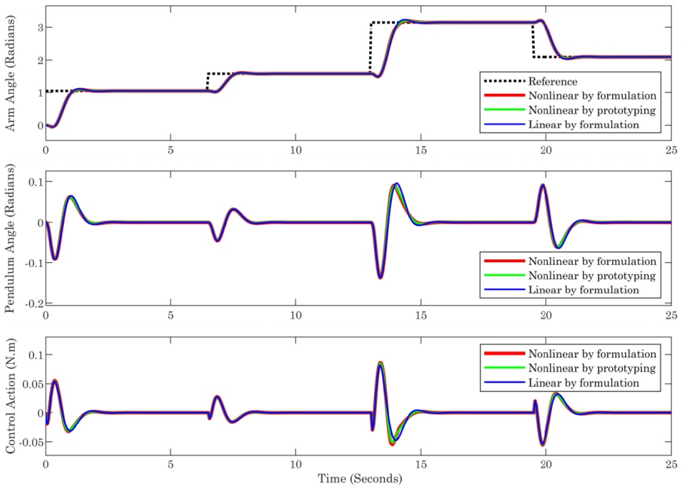
Now we apply the linear state-feedback control strategy (13) in three different models: (i) nonlinear dynamics as in (5); (ii) linear system as in (7) subject to (11); and (iii) virtual prototyping (Adams). We assume the initial condition x0= 0 0 0 0T for all the simulations.

We build the closed loop system of the two nonlinear models as follows. For the formulation model, the gains of equation (16) control the model shown in (5). The nonlinear model obtained with virtual prototyping is controlled through the gains of (17).

The resulting data taken from these three models are summarized in Figure 5. As can be seen, the three models generate similar responses, yet the response from the linear system seems to drift away from the other two during the transient time. As expected, the pendulum's angular position and the control action oscillate for a while and return to a steady state.

Figure 5 Simulated data. Three models were simulated with linear control (13) subject to (16). 

To prove the system's stability, we can mention that all the eigenvalues of the state matrix of the closed-loop augmented system contain a negative real part for the linear models. The eigenvalues of the linear model by prototyping are -2.5834+3.9166i,  -2.5834-3.9166i,  -9.3798+0.0000i,  -8.0587+0.0000i, and -4.1159+0.0000i. The eigenvalues of the linear model by formulation are -9.1022+0.0000i,  -8.1267+0.0000i,  -2.5483+3.9467i,  -2.5483 -3.9467i,  -4.1014 + 0.0000i . The local behavior of a nonlinear system near a linearization point is very similar to the behavior of the linear system at that point. It is precisely for this reason that we use the gains obtained for linearized systems in nonlinear models. Therefore, a nonlinear system can also be considered stable close to the linearization point.

The LQR+I control showed a good performance and low control effort, similar to that presented in ^{Hazem et al. (2020)} for the double-link rotary inverted pendulum system.

Remark 3: The three models for the Futura pendulum were extensively simulated using distinct profiles. In all simulations, we observed that the models remained stable. This numerical evidence suggests that.

In summary, the simulated data suggest that the linear state-feedback control (13) can stabilize the three models. This numerical evidence encourages using (13) for the Furuta pendulum in real time.

Remark 4: A video that shows the simulation in Adams was recorded and is available freely at https://youtu.be/w3Pg60J_3cM. This video illustrates the prototype of the Furuta pendulum moving its arms for distinct references according to the LQR+I control (13).

4. Conclusions

This paper has revisited the modeling and control of the Furuta pendulum. This paper documents how to obtain the nonlinear dynamics of the Furuta pendulum through the Euler-Lagrange formulation, following ^{Cazzolato and Prime (2011)}. The nonlinear dynamics then fed a linear model that has given rise to the linear feedback control. The linear feedback control was then applied to the nonlinear dynamics, the behavior of the nonlinear dynamics seems to agree with the one from the virtual prototyping Adams (see Section 3). Data from both models (i.e., nonlinear dynamics and virtual prototyping) suggest that the linear control can stabilize the Furuta pendulum. This fact motivates further research on how to design efficient, simple controllers to ensure the Furuta pendulum's stability. This paper, then, can be interpreted as a step in that direction.