2.1. Model analysis

The modal analysis was carried out to determine the natural frequency and corresponding modal shape at which the CMF should be forced to oscillate. Modal frequencies are usually obtained by solving the standard Eigenvalue equation (2.1).

where for a CMF, the external exciting force Ft is

Here, M, C, and Ҡ are the Mass Matrix, Damping Matrix, and Stiffness Matrix, respectively. F0 is the amplitude of excitation force, fd is the first natural frequency of the CMF while Δt is the time shift between the oscillations of the sensors.

2.2. Structure domain

The structure‘s motion is modeled by Hamilton’s variational principle, equation (2.3) as in (^{Rongmo & Jian, 2013}). It provides full information on the system's dynamics by the use of an action integral of a single function.

where WP and Wk are total potential energy and total kinetic energy. They are respectively represented by equations 2.4 and 2.5 (^{Mole et al., 2008}).

where p→s(x,t) the surface tractions acting upon the moving shell boundary through the respective displacement x→s(x,t) and F(t) is the driving force. Єs(x,t) and σs(x,t) are the strain and the stress tensor in the structure, and rp is the position vector of the point where the force Ft is applied. ρs is the structure material density and v→s is the structure velocity field.

2.3. Fluid domain

The governing equations for the fluid domain are the Reynolds-averaged Navier-Stokes (RANS). For the incompressible steady-state flow as follow, they are presented as equations (2.6) and (2.7):

where u- is the mean (streamwise) velocity of the fluid, u' is the turbulence fluctuations, ρ-F is the average density of the fluid, P- is mean pressure, µ is the dynamic viscosity and ρFui'uj'- is the Reynolds stresses.

2.4. Key parameters

The deformation (difference of displacement) of the meter (∆zCMF) can be calculated by equation (2.8).

where ∆t is the time shift between the oscillation of the inlet and outlet sensor points.

The time shift corresponding to the displacement at the locations of sensors (at the sensor at the inlet arm and the sensor at the outlet arm) is used to determine the mass flowrates of the fluid through the CMF. That is,

where

Here, K is the meter factor, L is the length of the CMF arm to the sensor and r is the radius of curvature of the CMF arm.

2.5. Modeling and simulation

This study considered a 3D CFD model of a U-shape CMF made of 316L stainless steel in Figure 1 for which properties are presented in Table 1. The volume of a single tube is 2.5368x10-0.005m3, while its mass is 0.20472 kg.

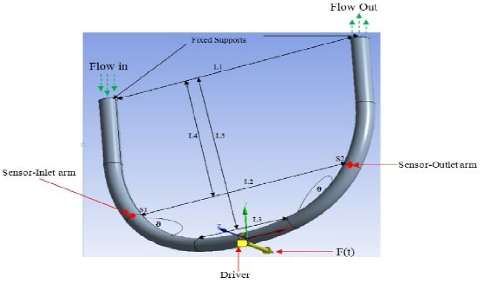
L1, L2, L3, L4, and L5 are lengths of different sections of a CFM, θ is the angle of bend of the CFM pipe while FM. The excitation force F(t) is indicated by a yellow arrow in the z-direction.

Figure 1 CFD model of a U-shape tube. 

The model analysis was conducted by using a mechanical ANSYS Parametric Design Language (ADPL) solver. The CMF’s tube was clamped at both ends and allowed to undergo free undamped oscillations. As a result of fixing the inlet and the outlet, the number of degrees of freedom for the tube reduces to 6.

The exciter was used to force the CMF’s tube to undergo undamped oscillations into the appropriate modal shape. These oscillations caused by the excitation force induce symmetric displacements of the CMF. Two motion sensors (S1 and S2 in Figure 1) were mounted symmetrically to the point where the excitation force is applied to detect and display these displacements.

For the fluid domain, FLUENT software was used. The Shear Stress Tensor k-ω turbulent model was chosen to solve the Reynolds-averaged Navier-Stokes (RANS) equations 2.6 and 2.7. Among the RANS turbulence models, the Shear Stress Tensor (SST) k-ω is deemed the most accurate and powerful. It combines the accuracy of the k-ɛ model in the free stream region and the excellent performance of a k-ω in the near-wall region.

Throughout the simulations, the velocities had been repeatedly varied at the inlet. The initial velocities corresponding to the selected sample of mass flowrates are presented in Table 2. In the table, NFR stands for nominal flowrate and ID is the inner diameter of the meter’s tube. For the current study, 14 different inlet velocities were considered. After separately carrying out simulations on structural dynamics and fluid dynamics both the dynamics were coupled to simulate the dynamics of the combined fluid-tube system.

3.1. Mass flowrates and meter error

The simulations were carried out on water with µ=0.001003 kg/m.s and ρ=998.2 kg/m³, Fuel Oil with µ=0.048 kg/m.s and ρ=960 kg/m³, Engine Oil with µ=1.06 kg/m.s and ρ=889 kg/m³, RME180 with µ=0.17838 kg/m.s and ρ=991 kg/m3, and RMG380 with µ=0.37658 kg/m.s and ρ=991 kg/m3. The temperature was kept at 27°C. The resulting mass flowrates are presented in Table 3. According to the table, the computed mass flowrates differ slightly from the baseline and there is no case in which the estimated mass flowrates are above the actual mass flowrates observed.

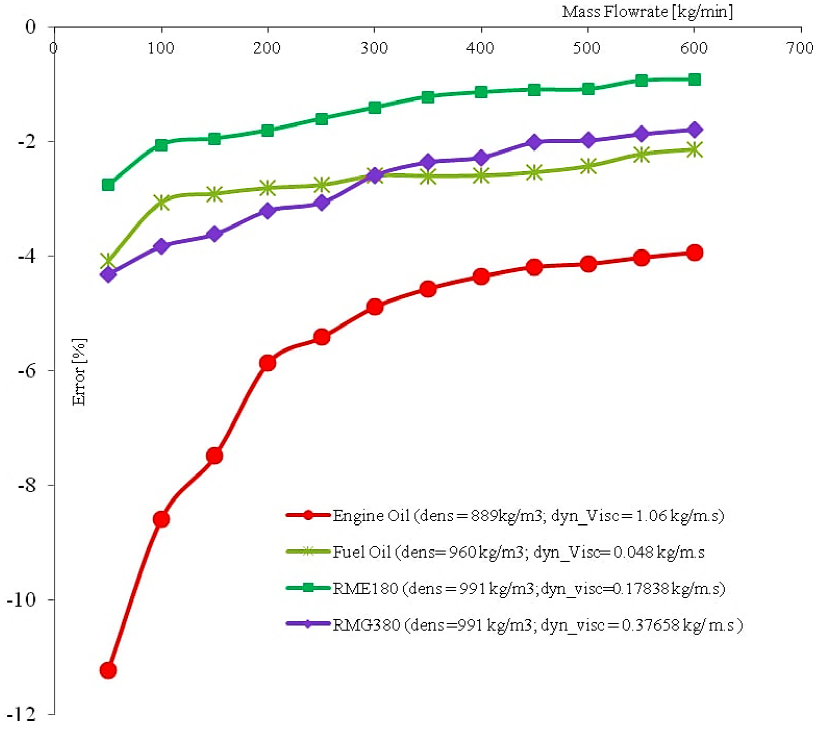
By a closer investigation of the error presented in Figure 2, the simulation predicts the error on computed mass flowrates that sharply decreases as the NFRs increase. For example, for Engine Oil with dynamic viscosity, µ=1.06 kg/m. s and density ρ=889 kg/m³, the error has decreased by about 65% as the mass flowrates increased from 50 kg/min to 600 kg/min. The change in density has no significant influence on the result. As can be noted, the deviation for RME180 with µ=0.17838 kg/m. s and ρ=991 kg/m³ and RMG380 with µ=0.37658 kg/m. s and ρ=991 kg/m³ differ despite having the same density.

Figure 2 Errors in mass flowrates. 

3.2. Sudden pressure increase

The sudden variation of pressure on the walls of the CMF’s tube may be one of the main causes of error growth as the viscosity of the fluid increases. Figure 3a-d plots the distribution of the total pressure on the walls of a CMF at each node from the inlet to the outlet. In Figure 3.a and Figure 3.c the pressures exerted by a highly viscous Engine Oil to CMF walls are plotted while in Figure 3.b and Figure 3.d the pressures exerted by water flow are presented. The dynamic viscosity of Engine Oil is 1.06 kg/m. s and is approximately 1000 times higher than the dynamic viscosity of water, i.e. 0.001003kg/m.s.

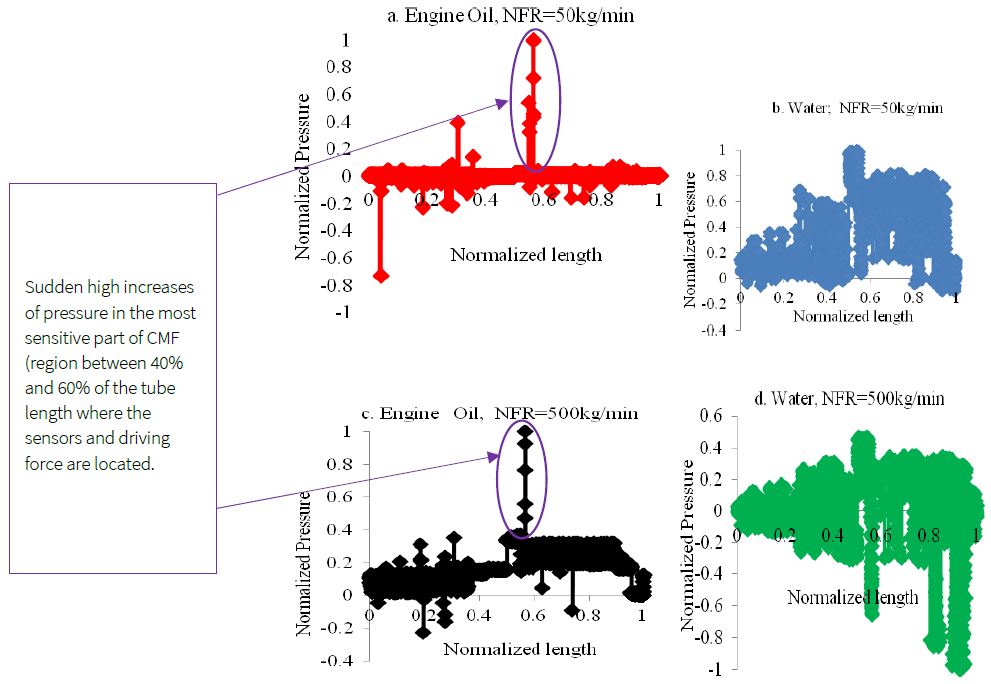
Figure 3 Pressure distribution on the tube’s wall along the CMF tube for fluid of different viscosities at different mass flowrates. 

As can be seen from the figures, the pressures of the water flow on the CMF remain fairly evenly distributed. In this, the influence of pressure on CMFs’ error remains as small as 0.01% to 0.13% per bar depending on CMF type/generation (^{Wang & Hussain, 2010}). Unlike water flow, for the highly viscous Engine Oil, the pressure largely increases suddenly in the vicinity of sensors (between 40% and 60% of the CMF length where the driving force and the sensors are located). The impulsive change of pressure in the more sensitive part of the CMF tube (near the location of the sensor at the outlet arm) likely lead to the outsized measurement errors. The sudden increase of pressure is likely to be associated with the occurrence of secondary flow. Various studies found that the secondary flow occurs due to low Reynolds numbers. Particularly, this study found that the reverse flow potentially due to high viscosity causes a sudden pressure raise near the sensor at the outlet arm S2, see Figure 1. When the flow reverses at the sensor S2, a part of the fluid returns towards the central part of the CMF mixing with the fluid flowing from the inlet causing the pressure surge in the section of the CMF just upstream of sensor 2 at the outlet arm as can be seen on Figure 3.a and Figure 3.c.

On the other hand, for water flow, the secondary flow of much lower magnitudes occurred in the central part of the tube, see Figure 4 and Figure 6. It is far from the sensors’ locations compared to the locations where the secondary flow occurred for the high viscosity flows. This results in a significant variation in pressure between the sensor at the inlet arm and the sensor at the outlet arm of the CMFs as can be seen in Figure 3.b and Figure 3.d. However, that variation of pressure is very low and not sudden compared to the change of pressure observed for high viscosity engine oil flow (Figure 3.a and Figure 3.c). Hence the associated deviation in the CMFs readings is insignificant compared to CMFs’ errors for measurement of high viscosity flow, Figure 2.

Figure 4 The flow of water through a CMF at 50kg/min-Streamlines 

Figure 5 Flow of Engine Oil, dyn-visc=1.06 kg/m.s through a CMF at 50 kg/min 

Figure 6 Flow of water, dyn_visc=0.001003 kg/m.s, through a CMF at 500 kg/min 

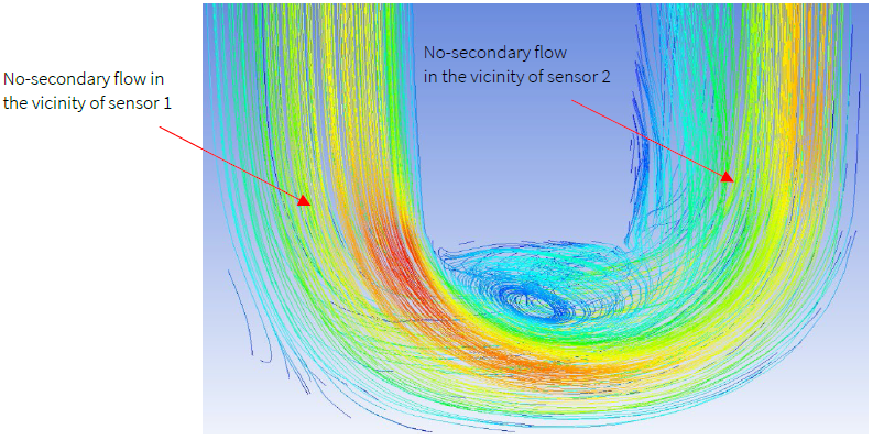
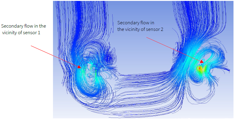
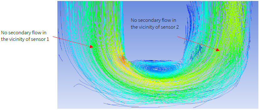
3.3. Secondary flow occurrence

Other than pressure jumps, the secondary flow near the sensors’ locations is another (even major) factor of the CMF’s error in the measurement of high viscosity flows. Figure 4 to Figure 7 present the flow patterns for water and Engine Oil. In Figure 4 and Figure 6, the streamlines indicate the flow pattern of pure water with dynamic viscosity at 0.001003 kg/m.s at a low nominal flowrate of 50 kg/min and a high nominal flowrate of 500 kg/min, respectively. On the other hand, Figure 5 and Figure 7 present the flow pattern for Engine Oil with high viscosity at the same aforementioned nominal mass flowrates. As the figures show, unlike for the low viscosity flows (pure water flow) where the secondary flow does form at the sensors’ locations, for the highly viscous flows the secondary/reverse flows occur at the sensors’ locations.

Figure 7 The flow of Engine Oil, dyn_visc=1.06 kg/m.s, through a CMF at 500 kg/min 

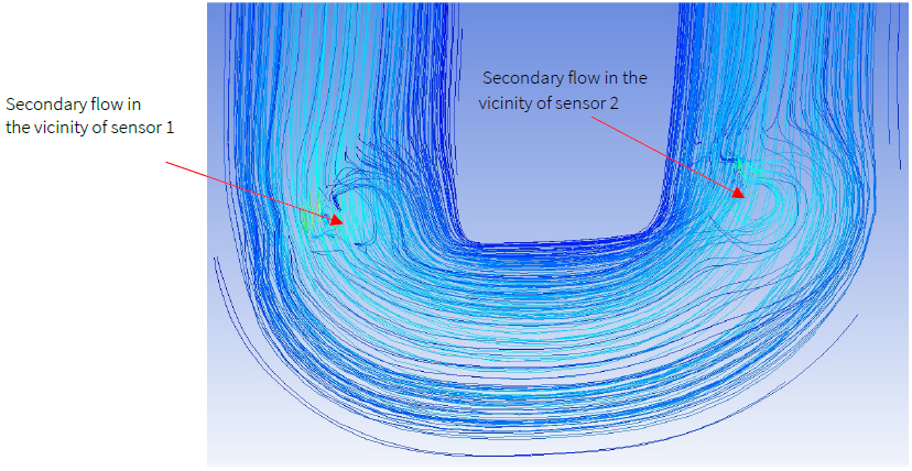
Due to secondary flow occurrence at the sensors’ locations, a part of the flow’s momentum diminishes in the reversed flow and does not contribute to the tube’s deformation. Hence, the deformation of the tube at sensors' locations is reduced, and therefore the CMF model reads lower masses of the fluid than its actual masses, hence large errors. This is supported by the findings of previous studies that also found that the occurrence of secondary flow leads to CMFs’ errors (^{Bobovnik et al., 2004}; ^{Kumar & Anklin, 2011}; ^{Mole et al., 2008}). The difference is that they attributed these errors to low Reynolds numbers only. It is to be noted that the decrease of the Reynolds number for a given fluid through a CMF of constant radius at a given radial speed is due to a change in fluid viscosity. Therefore, one can affirm that the error of CMFs on high viscosity fluid is dependent on fluid viscosity that causes the secondary/reverse flow. This finding is consistent with findings of other research on the measurement of low Reynolds numbers by Coriolis Mass Flowmeters (^{Huber et al., 2014}; ^{Kumar & Anklin, 2011}; ^{Rongmo & Jian, 2013}).