


 nueva página del texto (beta)
 Inglés (pdf)
 Artículo en XML
 Referencias del artículo
 Enviar artículo por email
 Citado por SciELO
  Similares en
SciELO
Similares en
SciELO 
 Permalink
1. Introduction
Milling is still one of the most used processes in manufacturing technology, it plays a crucial role in the field of mechanical manufacturing and, therefore, it is an open process to cope with various types of improvements. Because of the complexity and the optimization objectives, a large number of researches are guided towards new technologies in order to improve the productivity, the quality of the machined parts and minimize the production costs.
In the milling process, cutting parameters such as cutting speed, feed per tooth and depth of cut, as well as the cutting environment, material and tool geometry play a very important role in deciding the performance of quality.
To achieve the required quality performance, it is necessary to take into account an optimal selection of cutting parameters. This selection not only guarantees a reduction in costs and production times, but also guarantees control of the phenomena accompanying cutting, which directly affect the quality performance of the machined parts.
During milling operations, the part is heated by the phenomena associated with the formation of the chip and undergoes exchanges with the environment which results in high temperatures.
The cutting temperature causes heat generation and local heating linked to the tool-material pair present. These overheating lead to plastic deformation, during the formation of chips, and the increase in friction forces and the cohesion of the cutters on the cutting face. These overheating are local and strongly linked to the tool-material pair present. They can lead to the appearance of geometric and / or dimensional defects on the parts.
The heat generation mechanisms are linked to the plastic deformations generated in the primary shear zone by the conversion of a large amount of energy into heat and the secondary deformation at the chip-tool interface by the generation of heat by friction and / or shearing.
Increasing the cutting temperature during milling operations causes several problems, including rapid tool wear and thermal damage and fracturing of the inserts, which leads to a reduced service life and therefore a high production cost (Abukhshim et al., 2006; Majumdar et al., 2005; Young et al., 1996 ).
The increase in cutting temperature also affects the integrity of the machined surface and the dimensional accuracy of the workpiece.
Several relevant researches have been carried out on the cutting temperature during machining operations. This research can be divided into three main areas: experimental, analytical and numerical methods.
The experimental methods for measuring the cutting temperature during machining can be mainly classified into two groups: direct and indirect methods.
Indirect methods of locating high temperature points across the entire device and only provide post-processing information and calibration is tedious. The most widely used direct method for measuring cutting temperature in research is the thermocouple method (El-Wardany et al., 1996; Kitagawa et al., 1997; Le Coz et al., 2012; McFeron & Chao, 1958; Wang et al., 1968). This method consists in placing thermocouples as close as possible to the analysis area requested.
The advantage of thermocouples is the simplicity and flexibility of use for simple acquisition and this at lower cost, but this type of methods does not effectively give precise temperature values, it mainly depends on the position of installation of thermocouples. They also present enormous difficulties in mounting the measuring devices, especially when using rotary cutting tools.
Another type of direct method for measuring cutting temperature is infrared thermography (IR), which has become a widely accepted and mature monitoring tool, where temperature is measured without contact. This technique is used in some research to determine the cutting temperature:
(Saez-de-Buruaga et al., 2018) used infrared thermography to determine tool temperatures and thermal fields in near real time. In their study, the temperatures are measured on the side faces of the tool normal to the cutting edge. They then used analytical theories to calculate the tool / chip contact temperatures.
(Abrão & Aspinwall, 1997) used a single-color infrared thermometer to measure the cutting temperature during filming operations. In their work the emissivity has not been calibrated.
(Zhao et al., 2018) used a two-color infrared thermometer to measure the cutting temperature during the turning of the Inconel 718 with a ceramic tool. In this work, the authors tried to eliminate the emissivity effect in order to improve the authenticity of the measured cutting temperature.
(Sato et al., 2011) developed an infrared radiation pyrometer for measuring the cyclic cutting temperature under the cutting face of a milling tool.
(Soler et al., 2015) used an infrared camera to measure the tool / chip contact temperature. In this work the camera was placed orthogonally to the flow of the chip. The work presented by Soler et al. 2015 is based on an estimate of the heat distribution between the tool and the workpiece.
Despite the many advantages of this type of method, they remain linked to the calibration technique used, which in turn is linked by the estimation of emissivity.
Analytical methods based on the study of the mechanisms that affect cutting operations. Much research has been done with analytical methods for decades:
The work presented by Hahn 1951, Trigger and Chao 1951, on a semi-ifini medium, is based on the approach of the mobile heat source with explicit hypotheses. They assumed that the heat source was due to shear.
(Komanduri & Hou, 2001) followed the same steps as (Trigger & Chao, 1951; Hahn, 1951) but with the introduction of another heat source due to friction.
(Stephenson & Ali, 1992) used the green functions to solve a model that takes into account the cutting tool like a rectangular prism with a time-dependent heat flow.
(Feng et al., 2015) studied the cutting temperature by a thermal conduction model by introducing the fundamental principles of the milling process.
(Baohai et al., 2016) used an analytical model-based method to predict the cutting temperature during milling, taking into account the actual friction of the tool-chip interface and the cutting temperature drop phase.
(Radulescu & Kapoor, 1994) Calculated the cutting temperatures on the tool from a heat flow which takes into account convection in ambient air.
This type of method is affected by the shapes and geometries and the boundary conditions considered which must simplify in most cases which leads to imprecision of the results.
Numerical methods provide solutions for complex cases through known numerical methods for example: the finite element method (FEM) and the finite difference method (FDM).
In the literature there has been much research using numerical methods.
(Hoyne et al., 2015) applied the finite element method to determine the cutting temperature in the tool. The results of this study showed difficulties in determining the actual cutting temperature field.
(Strenkowski & Moon, 1990) developed a finite element model based on Euler's theory to predict the temperature distribution in the cutter, tool and workpiece during cutting operations.
(Lazoglu & Altintas, 2002) used the finite difference method to model the cutting temperature. This study addresses the effect of cutting parameters on the wear of cutting tools and the relationship between wear and cutting temperature.
(Jen et al., 2003) studied temperature as a function of time using a volume control method based on the conduction phenomena.
(Cui & Guo, 2017) used the finite element method to determine the average value of the transient temperature of the tool and to study the effect of the cutting parameters on the cutting temperature.
Numerical methods are difficult to simulate and require relatively long computation time.
From the literature search presented above it can be concluded that there is a need for the development of precise methods for determining the cutting temperature during milling. It is also clear that the development of models for predicting the cutting temperature during milling depends not only on the method used for modeling but also on the experimental procedure used. Most of the scientific work in this subject is based on data inspired by the literature, which requires experimental development for the measurement of temperature.
In most of the work carried out, the thermal camera and the two-color infrared pyrometer have been considered as useful means for measuring the cutting temperature. Unlike a pyrometer, a thermal camera not only determines the temperature but also tracks the evolution of heat in the tool and in the workpiece.
This is why, in this paper, on the basis of tests of measurement of the cutting temperature with a thermal camera, the effects of the cutting parameters on the temperature of the tool are predicted with an intelligent method based on a fuzzy inferences system. The prediction results obtained by this model have been verified by other experimental tests.
2. Experimental procedure
2.1. Materials and Equipment
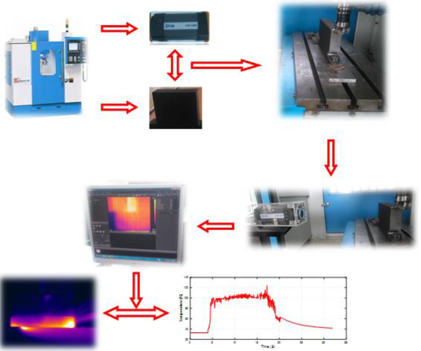
All milling tests were carried out under dry cutting conditions on a Knuth cnc mill Rapimill 700 type milling machine having a maximum spindle speed of 10,000 rpm and a maximum feed of 157 mm / min. Figure 1 shows the experimental configuration used.
The tests were carried out by surfacing prismatic parts in AISI 1060 carbon steel. The chemical composition of AISI 1060 carbon steel is described in table 1. A Sandvik 490R-08T308E-ML 1040 insert end mill was used to carry out all the tests.
2.2. Cutting temperature measurement
Measuring the cutting temperature in milling operations is too difficult due to obstructions to chips and the rotary movement of the cutting tool. Among the measurement techniques used for determining the cutting temperature during milling are: the infrared camera technique which is one of the most effective techniques. It has many advantages, such as: rapid measurement without contact with the heat source. With this method, the temperature is varied as a function of the thermal energy emitted by the surface of the body measured. However, the emissivity of a body depends on several factors such as: the emperature, the measurement configuration, the composition and the geometry of the surface measured, which makes the accuracy of this technique depends on the calibration technique used, essentially related to the estimation of emissivity. In addition, with infrared cameras, all materials do not have the same capacity to absorb or emit infrared energy by radiation: Emissivity. It is therefore essential to adjust the emissivity to adapt to the material to be measured to obtain a more precise measurement.
In this work, a FLIR A325 infrared thermography camera was used to measure the cutting temperature. In order to determine the emissivity, a matt black paint is applied to an area of the surface of the work-piece in order to display an emissivity greater than 0.95.
The temperature of the area thus painted is measured having set the emissivity to 0.95. At the end, the temperature of a neighboring surface located on the part is measured by modifying the emissivity until the same temperature is obtained.
The FLIR A325 infrared thermography camera is placed orthogonally to the flow of the chip, to measure the temperature on a side face of the tool. The measured temperature is the maximum cutting temperature. The configuration of the tests is presented in figure 1.
The experimental conditions used are presented in Table 2.
Table 2 Experimental conditions.
| Fz (mm/ tooth) | Vc (m/min) | a (mm) |
| 0.09 | 100 | 0.25 |
| 0.12 | 150 | 0.5 |
| 0.15 | 200 | 0.75 |
| 0.18 | 250 | |
| 300 |
The results of the cutting temperature measurement are obtained in the form of thermal radiation images. These images are analyzed by FLIR Tools control software to determine the maximum temperature of the cutting area.
2.3. Study of fidelity measurement system
In order to study the precision of our measurement system, we carried out temperature measurement tests, with the same cutting conditions three times in succession. Figure 2 illustrates the evolution of the cutting temperature for the three tests carried out.
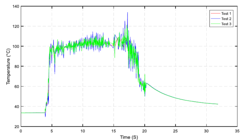
The results of the reproducibility tests are grouped in table 3.
Table 3 Result of reproducibility tests
| Tests | Temperature (°C) |
| Test 1 | 69.188 |
| Test 2 | 69.255 |
| Test 3 | 69.046 |
| Average | 30.3225 |
Standard Deviation 
|
0.087 |
The standard deviation is given by the equation (1)
The deviation is around 0.087 so the temperature values are grouped around the average, so it can be said that the temperature measurement is homogeneous for the three tests.
3. Results of experimental tests
Through tests carried out in this work, it is noticed that the cutting temperature increases with the increase in the cutting time, then it stabilizes and in the end it decreases when the machining operation is finished, which is clear in figure 3. This variation of the cutting temperature takes the same shape for all the tests and whatever the cutting parameters used.
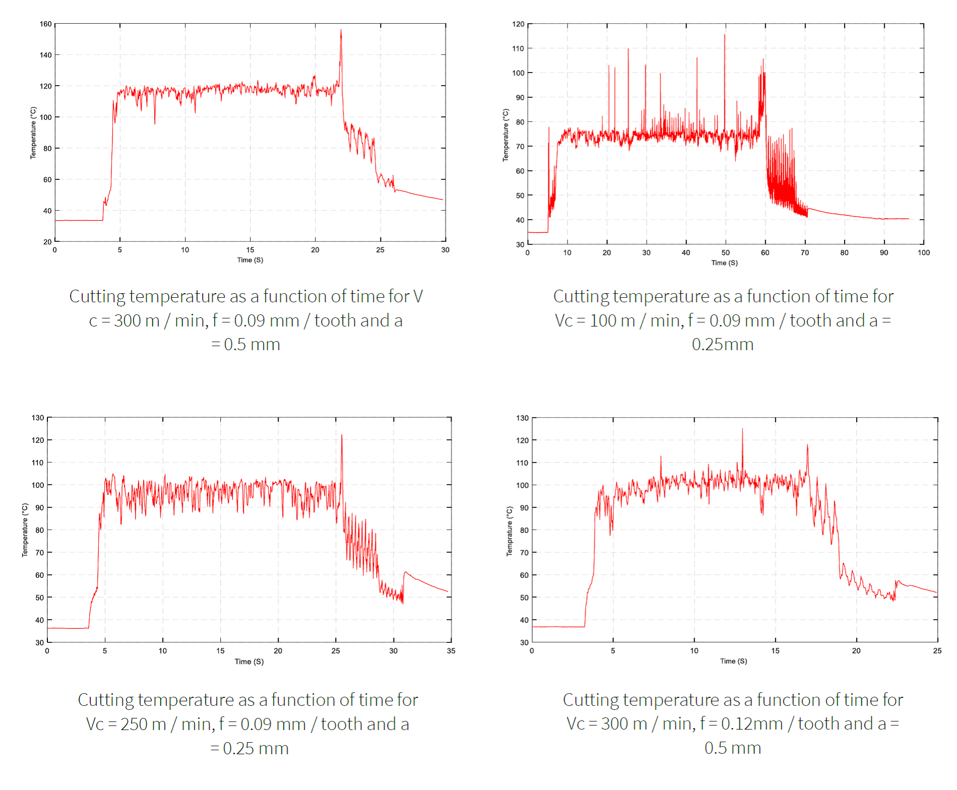
Each curve goes through three stages: an ascending temperature phase, then stability and finally the decrease in temperature.
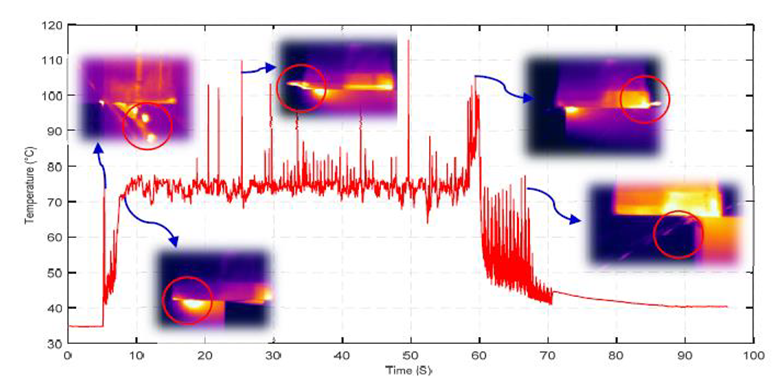
The peaks observed in the curve, intermittently, are the result of the crushing of the chips between the tool and the workpiece, which leads to an overheating of the chips, as illustrated by the thermographies appended to the curve of the Figure 4 (the zones of maximum temperature are surrounded by circles).
The study of the variation of the cutting temperature as a function of the cutting parameters leads to finding the values of the cutting temperature mentioned in table 4.
Table 4 Experimental results.
| a (mm) | 0.25 | 0.5 | 0.75 | |
| fz (mm/tooth) | Vc (m/min) | |||
| 0.09 | 100 | 74,73 | 101,00 | 91,55 |
| 150 | 91,62 | 101,50 | 117,80 | |
| 200 | 90,10 | 107,90 | 112,00 | |
| 250 | 99,54 | 114,60 | 125,50 | |
| 300 | 101,40 | 119,30 | 127,30 | |
| 0.12 | 100 | 79,23 | 88,59 | 105,40 |
| 150 | 85,59 | 98,96 | 114,10 | |
| 200 | 93,00 | 102,40 | 117,00 | |
| 250 | 96,65 | 109,40 | 120,80 | |
| 300 | 101,50 | 113,00 | 123,10 | |
| 0.15 | 100 | 78,46 | 86,33 | 104,20 |
| 150 | 83,90 | 97,00 | 112,20 | |
| 200 | 91,14 | 100,20 | 122,60 | |
| 250 | 94,49 | 102,90 | 118,10 | |
| 300 | 101,60 | 104,30 | 122,40 | |
| 0.18 | 100 | 80,39 | 88,83 | 103,00 |
| 150 | 84,25 | 97,83 | 110,20 | |
| 200 | 94,59 | 102,10 | 120,50 | |
| 250 | 91,50 | 102,90 | 123,00 | |
| 300 | 99,65 | 105,80 | 126,10 | |
4. Fuzzy model for milling
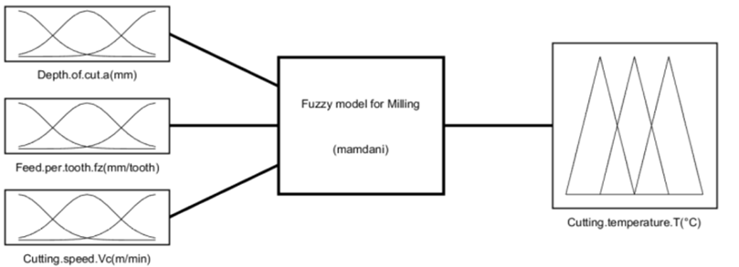
In this work, the fuzzy model designed to predict the cutting temperature for milling operations uses three inputs and one output (Figure 5). Cutting speed, feed per tooth and depth of cut are the inputs and the cutting temperature is the output of the system.
The process of the fuzzy logic technique gathers fuzzy logic operators, membership functions, managed by a set of rules. A fuzzy inference system is structured in three components: a fuzzy rule base; membership functions developed from a database; and a reasoning mechanism executing the rules to give an answer. The parameters used in fuzzy if/then rules define the fuzzy region of the inputs, while the output parameters provide the corresponding response.
The Mamdani type fuzzy inference system is used in this study.
Deux bases de données différentes sont utilisées pour le développement du système d’inférence flou ; une base de données est composée de 50 essais pour la conception du modèle flou, tandis que la deuxième base de données est composée de 10 essais pour la confirmation.
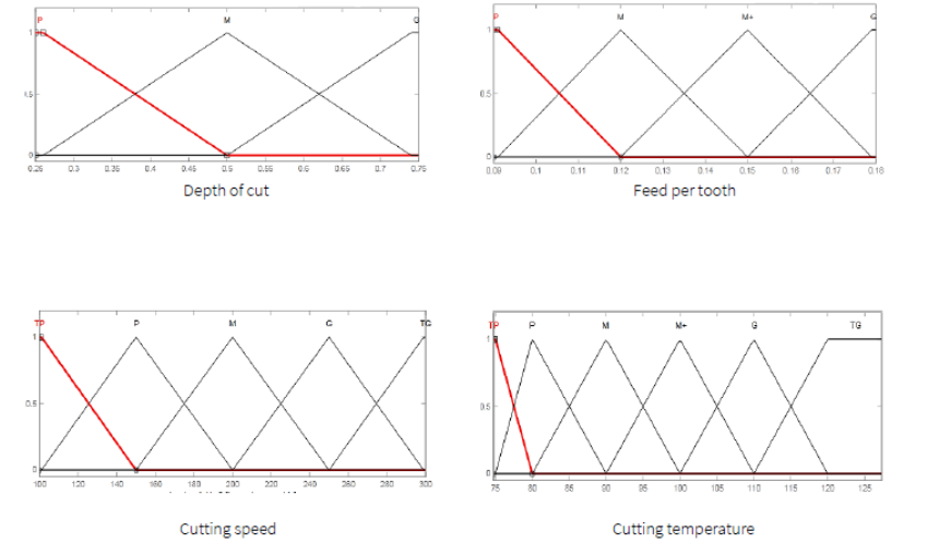
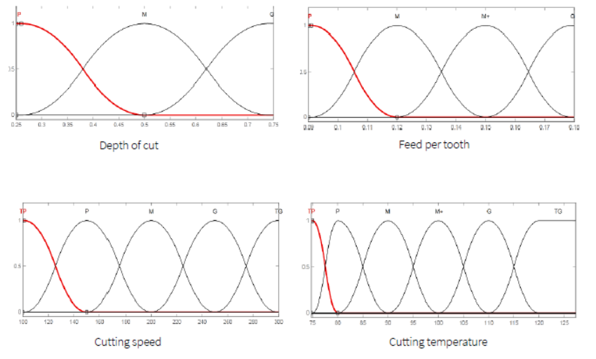
The first step in the study of the cutting temperature prediction algorithm is to choose the forms of the membership functions for the process variables according to the experimental database, which were used on the machine tool. Fuzzy expressions for cutting speed, feed per tooth, depth of cut, and cutting temperature are shown in Figures 6,7,8,9,10, respectively.


4.1. Fuzzy expressions
The numerical values of the input and the output are linked to a set of language variables, these connections are made by designing membership functions composed of several fuzzy values.
The numerical values of the depth of cut are linked by linguistic variables as shown in Figure 6.
The numerical values of the feed per tooth are linked by linguistic variables as shown in Figure 7.
Numerical cutting speed values are linked by linguistic variables as shown in Figure 8.
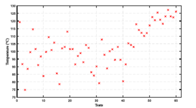
In order to determine the link between the numerical values and the linguistic variables associated with the cutting temperature, a representation in the form of a point (figure 9) cloud was proposed to determine the linguistic variables, taking into account the distribution of the values of cutting temperature obtained experimentally and ensuring optimal determination of the domain of each linguistic variable.
The numerical values of the cutting temperature are linked by linguistic variables as shown in Figure 10.

Membership functions come in many forms. In this study, triangular, trapezoidal and Gaussian membership functions were used for the input variables (cutting speed, feed per tooth and cutting depth) and the output parameter (Cutting temperature).
Six membership functions are used for the output response (cutting temperature). Increasing the number of membership functions leads to more accurate results, but at the same time, it leads to the use of a larger number of rules, which requires more computation time. Therefore, six membership functions were selected for this work. All fuzzy sets are defined by distinct membership functions. The output of the fuzzy inference system is visualized into fuzzy values that need to be defuzzified in the last step.
The triangular membership functions for the input and output parameters are illustrated in Figure 11.
The trapezoidal membership functions for the input and output parameters are illustrated in Figure 12.
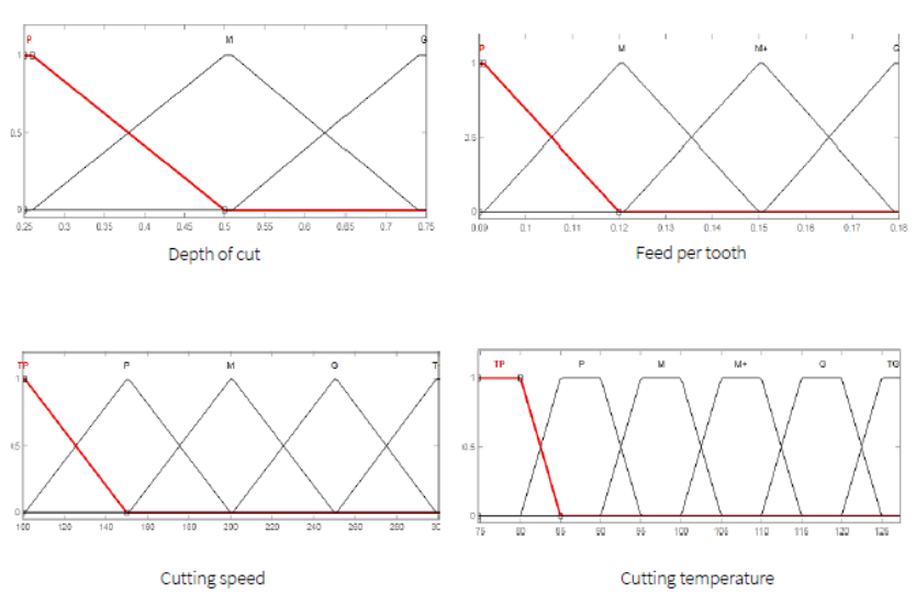
The Gaussian membership functions for the input and output parameters are illustrated in Figure 13.
4.2. Fuzzy rules for cutting temperature
The fuzzy model was created using fifty fuzzy rules defined on the basis of experimental work, among the sixty experiments carried out. The remaining ten experimental data will be used later to confirm the fuzzy model. The experimental database in Table 4 is used for the generation of the set of fuzzy rules. Table 5 illustrates the set of rules for the fuzzy system.
Table 5 Inference table.
| a (mm) | P | M | G | |
| fz (mm/tooth) | Vc (m/min) | |||
| P | TP | TP | M+ | - |
| P | M | - | TG | |
| M | M | G | G | |
| G | M+ | G | TG | |
| TG | - | TG | TG | |
| M | TP | P | - | G |
| P | M | M+ | G | |
| M | - | M+ | TG | |
| G | M+ | G | TG | |
| TG | M+ | G | TG | |
| M+ | TP | P | - | M+ |
| P | - | M+ | - | |
| M | M | M+ | - | |
| G | M | M+ | TG | |
| TG | M+ | M+ | TG | |
| G | TP | P | M | - |
| P | P | M+ | G | |
| M | M | M+ | TG | |
| G | M | M+ | TG | |
| TG | M+ | G | TG |
The fuzzy system created has three input parameters to produce an output, the fuzzy rules can be described in matrix form. Table 5 shows the set of matrix rules between cutting speed, feed per tooth, and depth of cut and corresponding cutting temperatures.
The first line indicates the fuzzy sets for the depth of cut (P: small depth, M: medium depth, G: great depth) from small depth to great depth. The first column indicates the fuzzy sets for the feed per tooth varying from low feed to high feed (P: low feed per tooth, M: average feed per tooth, M +: feed per tooth more than average G: high feed per tooth) , the second column indicates the fuzzy sets for the cutting speed varying from very low speed to very high speed (TP: very low speed, P: low speed, M: average speed G: high speed, Tg: very high speed) contents of the matrix is the result obtained, which is the cutting temperature for this study. The fuzzy operators used in the rules will apply are "" and "" and "" or "". Some examples of fuzzy rules in linguistic form are presented below:
1. If fz is (P: small) and Vc is (TP: very low) and a is (P: small) Then T is (TP: very low)
2. If fz is (P: small) and Vc is (TP: very low) and a is (M: average) Then T is (M +: more than average)
3. If fz is (P: small) and Vc is (P: low) and a is (P: small) Then T is (M: average)

50. If fz is (G: great) and Vc is (TG: very high) and a is (G: great) Then T is (TG: very high)
4.3. Defuzzification
The constructed model uses a continuous universe for all the input and output variables. So the input can be any combination of three variables (cutting speed, feed per tooth and cutting depth) and the output is the cutting temperature. Defuzzification makes it possible to merge the different rules generated by the inference engine to give it only one cutting temperature value and to transform this linguistic output variable into digital data by calculating the abscissa of the center of gravity of the membership function.
The output of the fuzzy inference system is defuzzified. The produced fuzzy sets are combined using aggregation operators from the input fuzzy rules. The fuzzy knowledge base system illustrated in Table 5 is trained based on expert knowledge, which leads to the generation of rules based on the experimental data in Table 4.
Centroid defuzzification method is used for defuzzification.
The results of defuzzification, which is the last step in fuzzy logic, are shown in Figure 14.
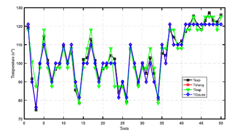
Figure 14 Variation of the experimental and predicted temperature as a function of the number of tests.
The results of the ten remaining experiments that did not enter the model creation process will be used to verify the model. These experiments were carried out under the same conditions as the previous experiments, but with different cutting parameters.
Table 6 groups together the fuzzy logic model predictions for the ten new tests.
Table 6 Confirmation tests.
| Tests | Cutting parameters | Cutting temperature | |||||
| Vc | fz | a | Texp | Ttriang | Ttrapez | TGauss | |
| 1 | 100 | 0,12 | 0,50 | 88,59 | 90 | 87,5 | 90 |
| 2 | 150 | 0,15 | 0,25 | 83,90 | 81,7 | 87,5 | 81,5 |
| 3 | 150 | 0,09 | 0,50 | 101,5 | 100 | 92,5 | 100 |
| 4 | 200 | 0,12 | 0,25 | 93,00 | 90 | 97,5 | 90 |
| 5 | 100 | 0,15 | 0,50 | 86,33 | 90 | 87,5 | 90 |
| 6 | 300 | 0,09 | 0,25 | 101,4 | 100 | 97,5 | 100 |
| 7 | 100 | 0,09 | 0,75 | 91,55 | 90 | 87,5 | 90 |
| 8 | 100 | 0,18 | 0,75 | 103,0 | 100 | 108 | 100 |
| 9 | 150 | 0,15 | 0,75 | 112,2 | 110 | 108 | 110 |
| 10 | 200 | 0,15 | 0,75 | 122,6 | 121 | 125 | 121 |
To choose between the membership functions of type: triangular, trapezoidal and Gaussian, we propose to use the standard deviation in order to define the values closest to the experimental results.
The standard deviation is given by the equation 2:
In our case N = 10 tests.
The standard deviation of the triangular membership functions is of the order of 2.2871
The standard deviation of the trapezoidal membership functions is of the order of 4.4359
The standard deviation of the Gaussian membership functions is around 2.3071
Then the results of the Triangular type membership functions are closest to the experimental results.
Study of the precision and the error of the fuzzy system.
To calculate the error percentage of the 10 tests equation (3) is used:
Equation (4) is used to calculate the percentage of the accuracy of the 10 tests:
The precision of the fuzzy model and the error rate are collated in Table 7.
Table 7 Fuzzy system error and precision for the ten verification tests
| Tests | Cutting parameters | Cutting temperature | |||||
| Vc | fz | a | Texp | Ttriang | Error % | Accuracy % | |
| 1 | 100 | 0.12 | 0.5 | 88.59 | 90 | 1.5916 | 98.4083 |
| 2 | 150 | 0.15 | 0.25 | 83.9 | 81.7 | 2.6221 | 97.3778 |
| 3 | 150 | 0.09 | 0.5 | 101.5 | 100 | 1.4778 | 98.5221 |
| 4 | 200 | 0.12 | 0.25 | 93 | 90 | 3.2258 | 96.7741 |
| 5 | 100 | 0.15 | 0.5 | 86.33 | 90 | 4.2511 | 95.7488 |
| 6 | 300 | 0.09 | 0.25 | 101.4 | 100 | 1.3806 | 98.6193 |
| 7 | 100 | 0.09 | 0.75 | 91.55 | 90 | 1.6930 | 98.3069 |
| 8 | 100 | 0.18 | 0.75 | 103 | 100 | 2.9126 | 97.0873 |
| 9 | 150 | 0.15 | 0.75 | 112.2 | 110 | 1.9607 | 98.0392 |
| 10 | 200 | 0.15 | 0.75 | 122.6 | 121 | 1.3050 | 98.6949 |
| Average accuracy | 97.7579 | ||||||
The Figure 15 compare the predictions of the fuzzy logic model with the temperature measured experimentally during the surfacing operation
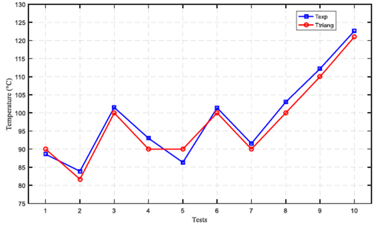
Figure 15 shows that the proposed model was able to accurately predict the cutting temperature during milling operations. The similarities between the cutting temperature values mean that the fuzzy logic model is an effective solution that can be used to predict the cutting temperature values for a specific range of cutting parameters.
The concordance of the results obtained by the fuzzy inference model developed with the experimental results re-reflects the correct choice of membership functions, the adequacy of the reasoning mechanism and the selected defuzzification method.
Table 8 illustrates a comparison of different works on the prediction of cutting temperature using empirical methods. From this comparison it is clear that the chosen technique succeeded in predicting the cutting temperature with a very low prediction error compared to the published works. Works that should be considered competitive with the literature are the RSM method of (Tamilarasan et al., 2016), the RSM method coupled with gray relational analysis of (Tamilarasan & Marimuthu, 2014) and Polynomial Regression by Ji et al. 2021, and the ANN-GA method of (Kumar et al., 2018).
Table 8 Comparison of different work on the prediction of cutting temperature.
| Authors | Modelling methods | Workpiece Material / tool material | Model parameters | Number of confirmation tests | Deviation (modeled / measured cutting temperature) | Remarks |
| (Sivasakthive & Sudhakaran, 2012) | RSM | Al-6060/HSS | Helix angle, Spindle speed, Feed rate, Axial depth of cut, Radial depth of cut | 0 | ~ 5% | The most influencing parameter is the helix angle |
| (Chawale et al., 2013) | Taguchi | Mild steel and cast iron/not specified | work piece metal, cutting speed, depth of cut, feed rate | 0 | Not specified | The most influencing parameter is the feed rate |
| (Al Hazza et al., 2012) | RSM | AISI H 13/coated carbide | cutting speed, depth of cut, feed rate | 0 | 9.6% | - |
| (Kovac et al., 2014) | Fuzzy logic | AISI 1060/ SPAN 12 03 ER (P25) | cutting speed, depth of cut, feed per tooth, Flank wear | 5 | 3.28% | The most significant factor on the cutting temperature is the depth of cut. |
| (Patel et al., 2014) | RSM | Mild steel/carbide | Cutting speed, Feed rate, Depth of cut | 0 | Not specified | The most influencing parameter is the depth of cut |
| (Sun et al., 2013) | Orthogonal array | Ti-6Al-4V/carbide | Cutting speed, Feed per tooth, Axial depth of cut, Radial depth of cut | 0 | Not specified | The most influencing parameter is the cutting speed |
| (Tamilarasan & Marimuthu, 2014) | RSM coupled with grey relational analysis | 11MnCrW4/coated carbide | Workmaterial hardness, Nose radius, Feed, Radial depth of cut, Axial depth of cut | 1 | 1.28% | The most influencing parameter is the feed rate |
| (Santhanakrishnan et al., 2015) | RSM | Al-6351/HSS | Rake angle, Nose radius, Cutting speed, Axial depth of cut | 0 | ~ 5% | The most influencing parameter is the cutting angle the effect of feed rate is not considered |
| (Tamilarasan et al., 2016) | RSM | 11MnCrW4/coated carbide | Cutting speed, Feed per tooth, Axial depth of cut, Radial depth of cut | 4 | ~ 0.64% | The most influencing parameter is the cutting speed and feed per tooth |
| (Pabst et al., 2010) | Polynomial regression | Grey cast iron/ Coated carbide | cutting speed, feed rate depth of cut, width of cut, rake angle, cutting edge radius | 0 | 3% | - |
| (Kumar et al., 2018) | ANN-GA | Al 6061 T6/ carbide | cutting speed, depth of cut, feed, step over | 4 | ~ 0.91% | The most influencing parameter is the depth of cut |
| (Zhu et al., 2020) | RSM | Stone-Plastic Composite | taper angle, spindle speed, feed rate, cutting depth | 1 | 4% | - |
| (Ji et al., 2021) | Polynomial regression | aluminum alloy 7050/ Ultrafine grained carbide | Cutting speed, Feed per tooth, Axial depth of cut, Radial depth of cut, Tool diameter, Blunt radius, Helix angle, Rake angle | 5 | ~ 1.6% | - |
| (Kumar et al., 2022) | GMEG-fuzzy | Inconel 625/ cemented carbide | cutting speed, depth of cut, feed, step over, Tool diameter | 5 | 5.85% | The most influencing parameter is the feed |
| Present study | Fuzzy logic | AISI 1060/ Sandvik 490R-08T308E-ML 1040 | cutting speed, depth of cut, per tooth | 10 | 2.24% | The most influencing parameter is the depth of cut |
However, fuzzy logic (the present study) outperformed the other methods because its high accuracy was proved by ten confirmation experiments, while the other methods were confirmed by five confirmation experiments at most which may affect its accuracy in case of an increase in the number of confirmatory experiments.
The high accuracy of the proposed technique was demonstrated by several different values of the cutting conditions.
4.3. Graphical representation of the fuzzy cutting temperature
Figure 16 shows a graphical representation of the fuzzy cutting speed as a function of the three cutting parameters.
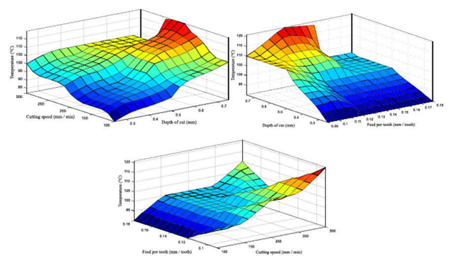
Figure 16 Variation of the temperature predicted by fuzzy logic according to the cutting parameters.
Figure 16(a) shows that the value of the cutting temperature becomes maximum for average values of the cutting speed (200 m / min) and maximum values of the depth of cut. While the minimum values of the cutting temperature are obtained for minimum values of the cutting speed and the depth of cut.
On the other hand, a higher depth of cut leads to an increase in the cutting temperature. Figures 16(a) and (b) show how the temperature increases due to the increased depth of cut regardless of the values of the other two parameters.
From Figure 16(b) we see that the value of the cutting temperature becomes maximum for high values of the depth of cut and minimum values of the feed per tooth.
Feed per tooth has a limited effect on the cutting temperature for minimum depth of cut values.
In figure 16 (c) the increase in the cutting speed leads to an increase in the cutting temperature regardless of the value of the feed per tooth.
The influence of the feed per tooth is not important, except for maximum values of the cutting speed.
The most important factor on the cutting temperature is the depth of cut. From FIG. 16 it is clearly observed that the depth of cut strongly affects the cutting temperature. The depth of cut has an increasing effect.
Conclusions
In this study, the infrared camera is used to accurately measure the cutting temperature in the cutting area as a function of time. The profile of the cutting temperature with the variation of the cutting time is recorded simultaneously. This experimental approach can be used in a practical way. It is useful to be an economical way to keep track of the cutting temperature of milling AISI 1060 steel with carbureted tools because it is easy to implement and use. The response of the measurement system to the nature of the milling operation is adequate and the results show that the cutting temperature and heat distribution were sensed satisfactorily regardless of the cutting speed used. In a second part of this study, a fuzzy inference model is developed to predict the cutting temperature during milling operations. The adequacy of the fuzzy model was checked and found to be adequate at an accuracy level of 97,757%, demonstrating that the model can be used to predict cutting temperature when milling AISI 1060 steel. The comparison and the validation of the fuzzy results with the results of the experimental tests confirmed the high accuracy of the model. The fuzzy modeling technique could be an economical and effective method to predict other parameters during milling operations based on cutting conditions. The results found showed that when machining AISI 1060 steel, the cutting temperature increased with increasing depth of cut and cutting speed while the feed per tooth had less influence. on the cutting temperature.

