


 nueva página del texto (beta)
 Inglés (pdf)
 Artículo en XML
 Referencias del artículo
 Enviar artículo por email
 Citado por SciELO
  Similares en
SciELO
Similares en
SciELO 
 Permalink
1. Introduction
Computational fluid dynamics (CFD) simulation is a costeffective alternative used to validate the performance of hydrokinetic turbines instead of conducting expensive experimental research (Tiwari et al., 2020). CFD studies, both two- and three-dimensional (3D) configurations, allow to simulate the flow around the turbine, calculate the blade forces, determine the velocity and the pressure distributions, predict the performance of the turbine of interest and study physical phenomena, including the flow separation and the geometry optimization of the turbine main components (Tian et al., 2018; Yavuz et al., 2015; Zhao et al., 2020; Zitti et al., 2020).
In order to numerically design a hydrokinetic turbine, the blade element momentum (BEM) theory or other approach is first employed to determine the hydrodynamic performance and the force generated on the turbine blades (Abutunis et al., 2019). Secondly, CAD model or computational domain of the turbine must be constructed. The third stage consists of dividing the domain into a finite number of cells by using a structured or an unstructured mesh. Afterwards, the Navier Stokes equations coupled with a turbulence model are used to build a mathematical model describing the changes on those physical properties for the fluid flow and the model geometry. Finally, several boundary conditions (e.g., velocity of the flow at the inlet, pressure, temperature and the density, among others), and a rotor rotation modeling approach are defined by the researcher in order to solve the problem throughout computer-based simulations. To verify the numerical simulations, mesh and time step convergence studies should be also performed. When a hydrokinetic turbine is numerically simulated, the flow domain consists of a dynamic and a stationary subdomain. Typically, the dynamic subdomain involves moving parts like the blades, rotor or moving surfaces. During the numerical simulation, each subdomain is independently discretized and then a boundary/interface is established in the surfaces that are in contact between each subdomain (Tian et al., 2018; Yavuz et al., 2015; Zhao et al., 2020; Zitti et al., 2020).
For the rotation modeling of the turbine rotor, several approaches such as the single moving reference frames (SRF) and the multiple moving reference frames have been proposed (Tabib et al., 2017). The SRF approach is used for modeling simple geometries when the computational domain is axi-symmetric. This method can be used when the computational domain is assumed to rotate. In the case of problems involving multiple moving parts, the stationary subdomain is discretized by means of the utilization of the stationary frame equations, whereas the dynamic subdomain is discretized using the moving reference frame equations. In ANSYs Fluent, there are two methods to treat the equations at the interface, such as the multiple moving reference frame approach and the sliding mesh model (SMM). Among the multiple moving reference frame approaches, the multiple reference frame model (MRF) and the mixing plane model (MPM) can be named (ANSYS Inc., 2018a). The referred approaches are steadystate approximations for treating the conditions at the interfaces. The MRF, which is widely known as the Frozen Rotor approach, is generally used when the flow at the interface is nearly uniform. In turn, the MPM allows to simulate the flow through domains containing one or more cells in relative motion. On the other hand, when the unsteady interaction between the dynamic and the stationary subdomains is important, the utilization of the sliding mesh approach is plausible to capture the transient behavior of the flow (ANSYS Inc., 2018b) In the multiple moving reference frames, the SMM is an accurate method for simulating flows; however, this method is more computationally demanding compared to other multiple moving reference frame approaches. In turn, when the mesh motion is a function of the solution or the mesh is deformed, the dynamic mesh method must be used along with the degrees of freedom (DoF) solver (ANSYS Inc., 2018b). It is highlighted that the dynamic mesh solution is intended to be more robust and accurate; nevertheless, it is also more time-consuming than other methods (ANSYS Inc. 2018b; Prakoso et al., 2019; Qu et al., 2015;).
In the literature, several studies reporting the use of the rotation modeling approach have been reported. As a matter of fact, Yavuz and coworkers utilized the MRF approach to define the blade rotation in order to study the performance of airfoil or hydrofoil arrangements for wind or hydrokinetic turbines, respectively (Yavuz et al., 2015). Similarly, Zitti et al. employed the referred approach to calculate the efficiency of Archimedes turbines (AST) (Zitti et al., 2020).
In contrast to MRF, the utilization of SMM has been reported by Tian et al. (2018) and Wang et al. (2019) to simulate the rotor rotation of a horizontal-axis hydrokinetic turbine. The simulations performed by Tian et al. were focused on the study of the wake structure and the flow around the blades (Tian et al., 2018). Concerning the numerical simulation conducted by Wang and coworkers, it was aimed at determining the force distribution along the blade (Wang et al., 2019). The MRF and SMM approaches for the rotating modeling are different from the experimental conditions, since the angular velocity (𝜔) and the rotation direction of the turbine rotor are boundary conditions that are defined in the setup of the problem, i.e., the hydrokinetic turbine rotor rotates around a particular axis at a certain 𝜔, which is previously set by the researcher, whereas this is a measured result under experimental conditions. To increase the precision in the results of the numerical simulation, 6 degrees of freedom (6-DoF) user defined functions (UDF) method is considered as an alternative approach since the turbine rotor ω is an output variable within the numerical simulation domain (Prakoso et al., 2020).
In turbo-machinery, the 6-DoF model has been commonly used to analyze systems as cross-flow turbines (Adanta, Budiarso et al., 2018; Adanta, Hindami &Siswantara, 2018; Prakoso et al., 2019; Siswantara et al., 2018), water wheel turbines (Adanta Budiarso, & Warjito, 2020) and open flume turbines (Adanta, Nasution et al., 2020). In hydrokinetic turbine rotor modeling, the 6-DoF approach has not been thoroughly investigated. From the authors’ knowledge, only the work carried out by Wang and coworkers was found to report the 6DoF model in the CFD simulation in order to evaluate the performance of a vertical-axis Darrieus turbine (Wang et al., 2011). Bouvant et al. (2021) reports an interesting work on the geometrical optimization of an AST as a hydrokinetic turbine. The results of the research were compared to the results available in the literature, providing significant improvement on the topic, especially on the methodology used for the optimization of the AST geometrical configuration. In the referenced research, the CFD numerical simulation was improved with respect to that one proposed by Zitti et al. (2020), when substituting the constant ω assigned to the turbine by a specific and a more realistic UDF function. Furthermore, the CFD results were extended with the use of the response surface methodology. This led to the identification of an optimal configuration, which was compared with other CFD, and experimental tests obtained from the literature.
It must be noted that Archimedes screw is an ancient technology and has been mainly used as a pump in several applications; nonetheless, in the last decades its use in different fields has been increased (Lisicki et al., 2016; Waters & Aggidis, 2015; Yu et al., 2016). While utilized in hydropower generation, AST allows to take advantage of water flows in sites with low heads and large flows to produce electricity (Dellinger et al., 2018). The use of the AST for electricity generation has a lot of technical, environmental and social advantages. The principal technical advantage is the high efficiencies achieved, from 60% or 80% (Hawle et al., 2012) to 92% in inclined-axis AST installations (ANDRITZ Hydro, 2012). Concerning the environmental dimension, this kind of turbine is considered as a renewable and an alternative energy source to carbon-based power generation systems, contributing to the reduction of greenhouse gas emissions. Moreover, these turbines are able to take advantage of kinetic energy as well as the water potential energy, leading to a minimal environmental impact. On the other hand, the AST generally operates at a low rotational speed, causing reduced morbidity and mortality to aquatic species (Kozyn & Lubitz, 2017). Finally, on the social side, AST can provide electricity to isolated communities with an acceptable investment, taking profit of its relatively low cost and simple construction. In addition, micro-hydropower would increase live quality. Furthermore, in areas near the national electric grid, the electricity generated by an AST could be supplied and sold, creating new opportunities and jobs (Madrid et al., 2015).
Under this scenario, in this study, a comparison between 6-DoF and SMM simulation approaches is conducted focusing on the performance of an AST prototype. Previous investigations had used only one approach to study the system rotation (Bouvant et al., 2021; Zitti et al., 2020). During the CFD simulations, Unsteady Reynolds Averaged Navier Stokes (URANS) equations coupled with the Shear Stress Transport (SST) turbulence model are considered. The validation of the numerical results is carried out by means of a case reported in the literature (Zitti et al., 2020) and experimental data obtained in the current work.
2. Materials and methods
2.1. Archimedes screw turbine geometry
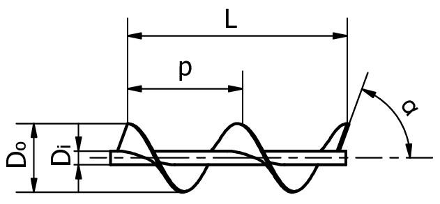
The main parameters taking part of an AST are the length of the shaft (𝐿), the number of blades, the blade pitch (𝑝), the diameter ratio (inner diameter/outer diameter, i.e., 𝐷𝑖/𝐷𝑜) and the inclination angle of the blade with respect to the axis (𝛼). These factors are shown in Figure 1. In this study, the AST parameters were set to be the same ones as those ones used by Zitti et al. (2020), so that the obtained numerical results were validated by using the experimental data reported in the referenced study. The AST parameters utilized in the conducted numerical studies are listed in Table 1.
2.2. Rotating models approaches
2.2.1. Sliding mesh model (SMM)
The SMM is a special and simplified case of the dynamic mesh model (DMM), where the nodes in the mesh are rigidly moved in a specific dynamic mesh zone. DMM allows to configure the relative movement of the boundaries in a cell zone (ANSYS Inc., 2018a). The solution process starts from a computational domain, which is subdivided into a moving and a static part, with respect to the basic frame of reference. These two domains are separated by the sliding interface to ensure a conservative distribution of the fluxes going from one subdomain to an adjacent one, as the mesh faces on each side do not usually match. In SMM, the mesh zone must be configured in a way that enables the non-conformal interfaces to be in permanent contact with each other. This is the reason it is called SMM, i.e., interfaces slide among them. The mesh moves like a rigid body (ANSYS Inc., 2018b), and even knowing that the mesh is moving in space, the nodes that define the cells do not deform it. A fixed rotational speed is imposed on the rotor by the SMM approach before solving the governing equations. Some examples of the use of SMM in numerical simulation can be found in Table 2.
Table 2 Reports concerning the use of SMM.
| Reference | Analyzed system | Goal | Setup | Concluding remarks |
| Bienz et al. (2003) | F1 braking systems | Improving aerodynamics in F1 cars | 3D numerical - MRF and SMM | SMM provided better results than MRF in braking systems analysis. |
| Dellinger et al. (2019) | Inclined AST | Comparing the performance of 3 AST with different number of blades and inclination | 3D numerical - Comparison with experimental results - SMM | Each analyzed turbine had a different optimal inclination. 5-blade AST showed the best performance. |
| Gullberg and Sengupta (2011) | Cooling fan for a car | Correctly simulating the efficiency of a cooling fan | 3D numerical - Comparison with experimental results - SMM and MRF | SMM described the system in a better way. MRF could not properly simulate the fan pumping capacity. |
| Gullberg et al. (2013) | Truck cooling fan | Presenting the correlation between simulations and experiments of axial cooling fans | 3D numerical - Comparison with experimental results - SMM | CFD simulations with SMM were able to predict, in an accurate way, the fan characteristic curve of the pressure rises. |
| Hobeika and Sebben (2018) | Vehicle wheel | Proposing an approach for improving the simulations of rotating wheels | 3D numerical - Comparison with experimental results - Proposed MRF grooves for rotating model | MRF grooves took advantage of the strengths of rotative wall model. MRF allowed to get satisfactory results in wheel system simulations without the computational cost ascribed to SMM. |
| Tabib et al. (2017) | Wind turbine at an industrial scale | Comparing rotating methods for wind turbine simulation | 3D numerical - MRF, SMM and RANS based actuator line | The rotating methods were compared to previous numerical results where the FAST methodology was used. The SMM showed the best results, followed by MRF and the RANS based actuator line. |
| Sammartano et al. (2016) | Cross flow turbine | Comparing turbulence models for the simulation and the design of cross-flow turbines | 3D numerical - Comparison with experimental results - SMM | Using SMM, the 𝐾−ɛ, 𝐾−ɛ RNG and SST-Kl turbulence models were contrasted. When comparing with experimental data, the best results were found using the SST-Kl model, followed by the 𝐾−ɛ RNG and the 𝐾−ɛ models. |
Note: Initials in table stands for: F1 (Formula 1), RANS (Reynolds -averaged Navier-Stokes equations), RNG (Re Normalization Group) and SST-Kl (Shear Stress Transport - Kato Launder production limiter).
2.2.2. Six degrees of freedom (6-DoF) method
The 6-DoF model has many capabilities and is used in simulations of different nature and complexity, since the 6DoF model utilizes the forces and moments acting on the body to know the actual movement state. In Equation (1), the translational movement for the center of mass of the body is calculated with respect to the inertial reference frame (ANSYS Inc., 2018a).
where
In turn, Equation (2) is used to compute the rotation movement of the body, applying body coordinates; where
The 6-DoF approach can be used to predict sequentially the angular positions according to the turbines mass properties (mass and moment of inertia) in real time. The 6DoF method computes the AST 𝜔 based on forces and moments acting on the rotor. Some examples regarding the application of the 6-DoF model can be found in Table 3.
Table 3 Reports concerning the use of the 6-DoF model.
| Reference | Analyzed system | Goal | Setup | Concluding remarks |
| Adanta, Budiarso and Warjito, (2020) | Water wheel turbine | Studying the effect of the channel inclination angle in the performance of the system | 3D numerical - 6- DoF | By performing simulations with 0, 10, 15, 20 and 25° of channel inclination, higher efficiencies were obtained with the channel at 10° of inclination. |
| Adanta, Nasution et al. (2020b) | Open flume turbine (OFT) | Analyzing and proposing the 6DoF method as a tool in OFT simulations | 3D numerical - 6- DoF | 6-DoF model was a great tool in the study of systems whose operating conditions depend entirely on their interaction with the fluid. The 6-DoF model in OFT simulations delivered better patterns than those ones in SMM. |
| Adanta, Budiarso, et al. (2018) | Cross-flow turbine | Comparing the system performance when using NACA and traditional profiles | 3D numerical - Comparison with experimental results - 6-DoF | Better results were found for the turbine designed with traditional blades. The 6-DoF model was used to obtain an adequate description of the turbine impeller rotation. |
| Go and Ahn (2019) | Tow-fish | Investigating the behavior of the system using CFD methods | 3D numerical - 6- DoF | Developing CFD simulations with the 6DoF model, linear and non-linear hydrodynamic damping coefficients could be determined more precisely than by using other methods. |
| Hopfe et al. (2013) | Throttleable Ducted Rocket (TDR) | Simulating the trajectory of a ramjet missile | 3D numerical - 6- DoF | The 6-DoF method used in CFD could calculate aerodynamic forces and moments significantly well and quite close to what would be obtained in experimental studies, leading to cost reduction. |
| Prakoso et al. (2019) | Cross-flow turbine | Comparing the system behavior while using the 6DoF and SMM methods | 3D numerical - 6DoF and SMM | Comparing with experimental results obtained by Sammartano et al. (2016), deviations of 6.8% and 12.4% were found for the 6-DoF and SMM simulations, respectively. |
| Qu et al. (2015) | Jet | Analyzing the emergency landing on water of a jet | 3D numerical - 6- DoF | The 6-DoF model allowed to study the behavior of the body while it is submitted to the impact forces. |
Note: initials in the table stands for NACA (National Advisory Committee for Aeronautics)
2.3. Numerical simulations
The performance curve for a hydrokinetic turbine is obtained by representing the power coefficient (𝐶𝑝) versus (vs.) the tip speed ratio (𝑇𝑆𝑅 or 𝜆). It is important to note that 𝐶𝑝 is the ratio between the power generated by the AST and the total energy contained in the flow passing through it. In turn, 𝜆 characterizes the AST rotational speed regarding the inflow velocity.
𝐶𝑝 and 𝜆 can be computed as described by Equations (3) and (4), respectively, where 𝑃 is the turbine power output, 𝜌 stands for the density of water, 𝐴 is the cross-flow surface of the turbine (𝐴 = 𝜋𝑅2), 𝑉 refers to the water inlet velocity and 𝑅 is the turbine radius.
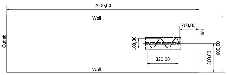
To compare the SMM and the 6-DoF models, the simulations were configured in the same way, the rotating speed the differentiating element. In each simulation, a rotating domain or internal domain (cylindrical body, which includes the turbine footprint) was defined, as well as a fixed domain or external domain (parallelepiped of length, width, and height equal to 2 m, 0.6 m and 1 m, respectively), which encloses the rotating geometry and contains the boundaries. The fixed domain was designated to represent a water channel, whose general dimensions and the dimensions of the rotating body are represented in Figure 2. The turbine shaft was positioned at 0.5 m from the top surface of the domain and at 0.3 m from each of the walls. The dimensions for the water channel representation and the AST geometry were the same as those ones reported by Zitti et al. (2020), aiming at achieving comparable results. The 3D CFD simulations were developed in a parallel mode with 16 CPU cores, configured in a LENOVO Thinkstation P520 and equipped with an Intel Xeon W2145 @ 3.7 GHz processor and a 64 GB RAM memory. Each time step was configured to be run for a maximum of 30 iterations with a criterion of convergence of 10−4 for all the residuals.
The entire set of simulations were carried out using ANSYs 19R3 and ANSYs workbench, allowing all the necessary steps to perform the simulation. The CAD geometry was generated in ANSYs design modeler and was then connected to the ANSYs meshing module. In turn, the generated mesh was imported in ANSYs Fluent.
The 𝐾−𝜔 SST turbulence model was used to solve the 3D transient Reynolds-averaged Navier-Stokes equations and the SIMPLE scheme was set for the pressure-velocity coupling. This turbulence model is commonly utilized for hydrokinetic turbine modeling since it has been demonstrated to have better performance for complex flows, including adverse pressure gradients and flow separations, as occurs in horizontal-axis hydrokinetic turbines. This turbulence model offers an improved prediction of adverse pressure gradients in the near wall regions when compared to standard 𝐾−𝜔 and 𝐾−𝜀 models (Menter, 1994). The 𝐾−𝜔 SST turbulence model has been widely adopted by several researchers for the design of hydrokinetic turbines (Chitrakar et al., 2020).
For the channel inlet, considering that rivers in developing countries do not usually have flow velocities higher than 2 m/s (Andreadis et al., 2013), a velocity inlet of 1 m/s was used. For this boundary condition, a default turbulence intensity of 10% was implemented. At the domain outlet, a relative pressure of 0 Pa and a backflow turbulent intensity of 5%, was imposed as the pressure outlet boundary condition. For the walls (including the AST surface), no slip shear condition was enabled.
For the SMM simulation, 𝜔 of the rotating body (including the turbine footprint) was varied from 1.2 rad/s to 24 rad/s, with steps of 1.2 rad/s. Under this 𝜔 range and considering the inlet velocity of 1 m/s, a 𝑇𝑆𝑅 range between 0.06 and 1.2 was analyzed. Such 𝑇𝑆𝑅 range leads to a good representation of the AST performance curve. For the 6-DoF simulation, the angular position of the rotating body was registered during each time step, making possible to compute the instantaneous 𝑇𝑆𝑅 and to achieve a performance curve in the same range as in the SMM simulation.
For the 6-DoF simulation, the AST footprint and the entire domain were allocated in a way that with the water coming from +X to -X, the generated momentum would make the turbine rotates around the +X axis (one DoF rotation); the inertia tensor for the 6-DoF UDF configuration was computed with the help of SolidWorks software. The AST is limited to rotating around the X-axis, while the other DoF is not available. The specifications of the AST, which depend on the geometry and material of the turbine, are shown in Table 4. Small values of the moment of inertia promote the startup of the AST. However, excessively small values will impair the stability of the AST rotor rotation. For determining the moment of inertia, iron cast was selected, and the material density was 7150 Kg/m3.
Table 2 Specification of the 6-DoF body.
| Parameter and units | Value |
| Mass [kg] | 1.107 |
| Moment of Inertia [kg m2] | 0.00047 |
| Initial 𝜔 [rad/s] | 0 |
| Initial center of mass (x, y, z) [m] | (-0.173, 0, 0) |
Once the configuration was completed and the simulation was run, the 6-DoF model began to accelerate the body because of the interaction between the fluid and the turbine walls, and the 𝜔 rose to a stable and maximum value. From that point, a pre-load was set to the 6-DoF UDF, and the turbine slowed down until the condition of 0 rad/s was reached. The collected data from the imposition of the preload allowed to draw the 𝐶𝑝 vs. the 𝑇𝑆𝑅 curve. As the simulation has only one rotational DoF, it was not necessary to employ any of the mesh methods found in the setup of dynamic mesh options of Fluent software; that allows to define the rotation body as a rigid body whose rotational movement depends on the total momentum acting over the footprint surface. To ensure the correct transfer of information between the stationary and the moving domains, an interface boundary condition was employed, which also facilitated convergence.
2.3.1. Mesh independence
Mesh independence study is conducted in order to achieve a mesh with several elements that gives results close to reality and keeps a reasonable computational cost. As the 6-DoF simulations require better discretization conditions than the SMM simulations, the convergence studies were carried out to the numerical simulation results obtained by the application of the 6-DoF method. The mesh and time step configurations under which the results convergence is achieved were also utilized for the simulations using the SMM approach. Due to the complex geometry of the AST, an unstructured-tetrahedral mesh was created for the entire domain. Additionally, in order to determine the influence of the spatial discretization, the Richardson extrapolation method was used. For this purpose, three different meshes were created and named coarse, medium and fine mesh. The target parameter for the comparison of the meshes was the area under the curve formed by representing 𝐶𝑝 vs. 𝑇𝑆𝑅. The Richardson extrapolation is based on Taylor’s series and allowed us to obtain an improved estimate of the numerical result in derivatives, integrals or differential equations (Richardson, 1911). The generalized Richardson extrapolation was well presented by Roache (1994), standing a way to estimate the error associated with the spatial discretization in CFD simulations, which is considered as one of the numerical error main sources. This method has been successfully used in several CFD studies. For example, Prakoso et al. (2019) and Siswantara et al. (2018) applied the Richardson extrapolation in order to analyze the Grid Convergence Index (GCI) for the domain of a cross-flow turbine. In turn, Franke and Frank (2008) used the mentioned procedure to analyze its suitability for problems related with computational wind engineering, achieving good results.
One of the benefits ascribed to the Richardson extrapolation is the possibility of computing an estimate of the exact value (f0) for the analyzed variable, i.e., without the error due to the discretization. In order to calculate f0, the convergence coefficient (𝑃) must be calculated using the expression presented in Equation (5), where f3, f2, and f1 are the area under the curve of the coarse, medium and fine mesh, respectively. For the rest of the section, the sub-indexes 3, 2 and 1 stand for the coarse, medium and fine mesh, in that order, being established a normalized grid spacing. A helpful step in the calculus of 𝑃 is the estimation of the difference for the solution variation between meshes. The calculus of the above-mentioned parameter is obtained as described in Equations (6) and (7).
Once 𝑃 has been calculated, the estimate of f0 is possible to be determined, as shown in Equation (8). The term r refers to the grid refinement ratio and could be calculated as 𝑟 = ℎ3/ℎ2 = ℎ2⁄ℎ1, where ℎ𝑖 is the number of elements in each mesh. Although in this study the value of 𝑟 is not constant, 𝑟 is assumed to be equal to 2, since this value is near to the one in the meshes used and is higher than 1.3, representing the minimum value found by Roache (1998), under which good results were obtained.
An additional and widely used concept is the Grid Convergence Index (GCI), which brings an assessment of the discretization error among meshes. Equations (9) and (10) represent the way in which the GCI is calculated for each pair of mesh. In the referred equations, 𝐹𝑠 refers to a safety factor, which was set at 1.25 (Xing & Stern, 2010).
Finally, the results obtained within the used meshes must be checked to be in an asymptotic region of convergence. For this purpose, Equation (11) is used. A value close to 1 is expected to be achieved.
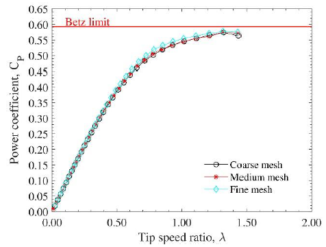
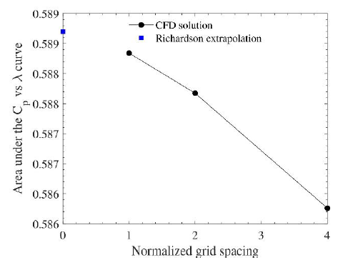
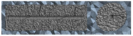
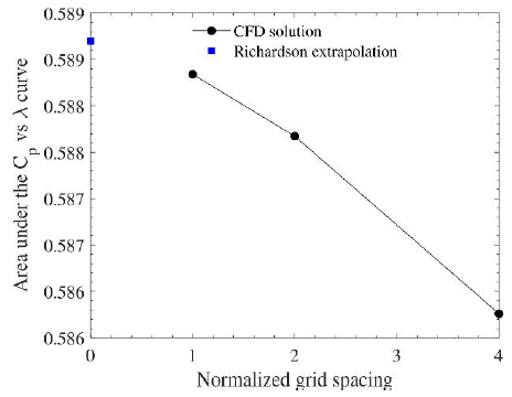
Figure 3 shows the results of the simulations (the evolution of 𝐶𝑝 vs. 𝑇𝑆𝑅) conducted during the mesh independence test. For the number of elements used, the variation in the results due to the number of elements in the mesh can be observed to be not significant. In Figure 4, the asymptotic tendency of the results obtained with the used meshes is illustrated. This agrees with the value of 𝐼 = 1.0011, which was obtained for the asymptotic convergence analysis. The 𝐺𝐶𝐼23 and 𝐺𝐶𝐼12 values were 0.22% and 0.076%, respectively, showing that the grid independence was achieved. Thus, the medium mesh was selected for the study simulations. Medium mesh was set with a first layer thickness of 1.58𝑥10−3 m, value that allowed to obtain a maximum dimensionless wall distance (y+) of 90.37, which is found in the range of 30 and 300, making possible to use the wall functions approach (Nieto et al., 2015).
Details for the different meshes are presented in Table 5. The meshes exhibited excellent quality parameters and the errors between the mesh results were less than 1%, which is also a also good indicator of convergence. A representation of the medium mesh used in the numerical study is illustrated in Figure 5.
Table 3 Mesh independence test.
| Parameter | Mesh | ||
| Coarse | Medium | Fine | |
| Number of nodes | 42873 | 82130 | 153303 |
| Number of elements | 218100 | 419907 | 794911 |
| Max skewness | 0.659 | 0.651 | 0.642 |
| Max aspect ratio | 4.698 | 3.894 | 4.838 |
| Min orthogonal Quality | 0.341 | 0.349 | 0.358 |
| Error with respect to the fine mesh | 0.325 | 0.113 | - |
2.3.2. Time step independence
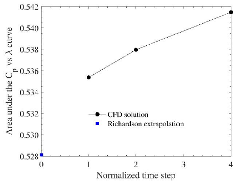
As in the mesh independence study, the time step independence was developed by using 6-DoF simulations. The Richardson extrapolation process was adapted to analyze the time step influence on the simulation results; the test was carried out for three different time steps (0.00025 s, 0.0005 s and 0.001 s) and in order to find the convergence time step Index (CTI), the analyzed time steps were normalized to be 1, 2 and 4, respectively. CTI is the reciprocal of the GCI (Prakoso et al., 2019) and in this study, a value of 2% or less for the CTI was chosen as a criterion of selection for the definitive time step. The 𝐶𝑝 vs. 𝜆 curves for each of the above-mentioned time steps are represented in Figure 6. Little differences could be observed at the end of the curves; however, a general good concordance in the data behavior was also found. CTI12 and CTI23 were 1.69% and 2.28%, respectively; satisfactory results for CTI were noted in the scale of Figure 7, which covers a variation of less than 0.014. A time step of 0.0005 s was used in all the simulations. Additionally, when analyzing asymptotic convergence for the time step, a value of 0.9952 was obtained. This value is close enough to 1 as to consider that the selected time step is in the asymptotic convergence region.
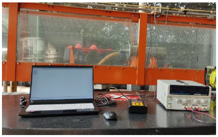
2.4. Experimental setup
Experimental tests were conducted in a hydraulic channel. The channel has a cross-section of 0.30 m x 0.45 m, with a length of 7 m. The water circulates through the channel with the help of centrifugal pumps, which are controlled by variable speed drives that allow to control the flow of water circulating through the system. For the tests, a target flow rate of 0.53 m3/s was established. At this flow rate, a speed of 0.5 m/s was obtained for the water in the channel. The velocity of 0.5 m/s was verified with a flow watch air and water speed flow meter (FW450 with a resolution of ±0.01 m/s). The turbine was 3D printed with fused deposition modeling, using a layer thickness of 0.2 mm and polylactic acid (PLA) as the printing material.
To measure the power generated by the turbine, a torque sensor Futek TRS 605-FSH02057 with encoder was used. This device has measurement ranges of 0-50 Nm and from 0 to 7000 RPM. The sensor is connected to the rotor and to the DC motor. The motor is energized so that its direction of rotation is opposite to that of the turbine, simulating the load of an electric generator and allowing operating data to be obtained at different ω.
The other components of the measurement and data collection system correspond to mechanical couplings, a watertight casing and supports of the system. In Figure 8, the setup used for the characterization of the turbine is illustrated.
3. Results and discussion
The final simulations were developed with a mesh of 419907 elements, a time step of 0.0005 s and a water velocity of 1 m/s. Figure 9 shows the results when each one of the rotating models was used. As observed in the figure, a significant difference in the AST performance curve is evidenced. A maximum 𝐶𝑝 of 0.574 at a 𝜆 of 1.319 was found utilizing the 6-DoF model, in comparison with the maximum 𝐶𝑝 value achieved using the SMM model (0.2755 at a 𝜆 of 0.78). The results obtained with the SMM approach are close to the numerical results presented by Zitti et al. (2020), since the referenced authors achieved a maximum 𝐶𝑝 of 0.238 at a 𝜆 of 0.75 with a water velocity of 0.2 m/s, which is a significant lower value for this parameter. Furthermore, concerning the difference obtained in 𝐶𝑝, it is important to note that Zitti et al. (2020) used the MRF method for the rotation of the turbine, which is less accurate than the SMM method (Gullberg & Sengupta, 2011; Hobeika and Sebben, 2018; Tabib et al., 2017).
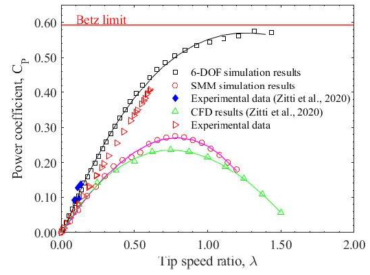
Figure 9 Comparison of rotating models and experimental data. Power coefficient (Cp) vs. tip speed ratio (λ).
In Figure 9, the experimental data are found to be better described when the 6-DoF model is employed. The fit of the SMM results is like those ones presented by Zitti et al. (2020), being the experimental data larger than those ones obtained from the simulations. The referred authors found an explanation in the flow confinement. Nevertheless, considering the better fit of the simulation data obtained by the 6-DoF method, the error associated with the utilization of the rotating model seems to be the most probable cause.
For 𝜆 values less than 0.4, the experimental data obtained are in the middle of the results for the 6-DoF and SMM simulations. However, when the rest of the points are analyzed, the data provided by the 6-DoF method are the closest to a greater number of the experimental data obtained.
The solid lines in Figure 9 correspond to cubic fits conducted to each one of the CFD simulation results. The equations for the regressions are listed in Table 6.
Table 4 Cubic fits for CFD results.
| Data | Cubic fit | R2 |
| 6-DOF simulation results. | 𝐶𝑝𝑑𝑜𝑓 = 0.0914∗𝜆3 −0.5966 ∗𝜆2 +1.07∗𝜆 −0.01321 (10) | 0.9989 |
| SMM simulation results. | 𝐶𝑝𝑠𝑚𝑚 = −0.106∗𝜆3 −0.269 ∗𝜆2 +0.624∗𝜆 −0.00232 (11) | 0.997 |
| CFD results (MRF) (Zitti et al., 2020). | 𝐶𝑝𝑚𝑟𝑓 = 0.0656∗𝜆3 −0.5166 ∗𝜆2 +0.6653∗𝜆 (12) | Non- registered. |
The discrepancies between experimental and numerical results can be caused by several factors. As a matter of fact, the bearing frictional losses of the turbine and the effect of the support on the flow field were not included in the simulation. Additionally, the support used in the experimental test can produce an effect on the AST hydrodynamic performance. The numerical results have smaller values compared to the experimental ones.
4. Conclusions
The results obtained in this study showed a good concordance with the information reported in the literature. In this regard, the behavior of the AST system was described in a better way when the 6-DOF model was used.
Even though a higher precision was found by using the 6DOF method, the SMM method continues to be a valuable option for the development of CFD analysis of hydrokinetic turbines. The SMM method can be used in order to estimate specific operation points with less computational cost, leading to faster design processes. In turn, the 6-DOF method could be a good option to be employed in the last stages of the turbine design, as more reliable data are needed. On the other hand, when a complete estimate of the turbine performance curve is required, the 6-DOF method could work it out in a shorter time, since by using the SMM method each operation point must be set and computed until good convergence conditions are reached.
When comparing the MRF simulation results obtained by Zitti et al. (2020) with those ones achieved in this study, the MRF approach seems to be a better approach than the SMM method; however, there are few experimental points for the comparison. Additionally, these few points are in a region where the SMM method has slightly better behavior. Therefore, the SMM approach is still considered as a better approximation method than the MRF approach. When compared with the other methodologies, the 6-DoF simulation was observed to be closer to the experimental data.
Further experimental research is needed to discern the real behavior of the AST turbine under working conditions. The results of these investigations would allow us to validate the simulation methods used here and select the most suitable one for the study of this type of turbine.

