Introduction
Mezcal, one of México’s emblematic drinks, is produced by the distillation of cooked and fermented agave juice (Espejel- García et al., 2019; Nolasco-Cancino et al., 2022). It can be produced with wild or cultivated maguey. Although the terms agave and maguey are used interchangeably, the term maguey refers to a wild plant and agave when it is cultivated (Hernández-López, 2019).
For the elaboration of mezcal, different species of mature agaves are used depending on the place of production, including Agave angustifolia and Agave potatorum in Oaxaca (Vera-Guzmán et al., 2018), Agave durangensis in Durango (Barraza-Soto et al., 2014), Agave salmiana in San Luis Potosí (Godínez-Hernández et al., 2015), Agave cupreata in Guerrero and Michoacán (García-Mendoza, 2012), Agave tequilana in Zacatecas (López-Nava et al., 2012), and Agave karwinskii in Puebla and Oaxaca (Vázquez-Pérez et al., 2020). Despite the distribution of agaves throughout mexican territory, only nine states have the Denomination of Origin for mezcal (DOM) (Hernández-López, 2018). In addition to the aforementioned states, Tamaulipas and Guanajuato also have DOMs (Vera-Guzmán et al., 2010). Depending on the elaboration process, the Mexican normativity classifies the mezcales as artisanal, ancestral, and mezcal (Dirección General de Normas, 2016). The relevance of mezcal can be seen in its production volume, from 1 million liters in 2012 to 8 million in 2021 (COMERCAM, 2022), which means a sevenfold increase in 9 years. Therefore, it becomes an economically valuable product, together with the cultural, environmental, and technological impact that it generates in the production areas (Rios-Colín et al., 2022).
However, mezcal is a highly susceptible beverage to adulteration because it can be easily mixed with cheaper liquids (Esteki et al., 2018), which compromises its authenticity, quality, and value in the market, consequently increasing the risk to consumer health (Tabago et al., 2021). This leads to the proposal of strategies to monitor the safety of alcoholic beverages consumers, as it is estimated that approximately 40 to 50 % of the beverages consumed in Mexico are illegal and clandestine (Gaytán, 2018). In this context, new metabolomics-based approaches are being implemented to analyze the quality of spirits and their adulterations (Gougeon et al., 2018). This requires knowledge of two scientific fields such as analytical chemistry and multivariate statistics (Fernandez-Lozano et al., 2019).
Infrared (IR) spectroscopy is a non-destructive, sensitive, fast (30 samples/hour), powerful, environmentally friendly instrumental technique that is widely used to analyze spirits (Arslan et al., 2021; Lachenmeier, 2007; Yadav and Sharma, 2019). In beer, mid-IR (MIR) spectroscopy has been used to determine authenticity (Lachenmeier, 2007), evaluate quality parameters (Llario et al., 2006), and control sugar production during maceration (Almeida et al., 2018). In wine, compositional parameters (glucose, fructose, pH, volatile, and titratable acidity) have been evaluated by MIR spectroscopy (Cozzolino et al., 2011). Cavaglia et al. (2020) also used this technique to detect, monitor, and correct bacterial contamination in white wine process. Finally, the MIR technique was used to predict sensory attributes of South Australian geographical indication (GI) wines (Niimi et al., 2021).
In agave spirits, Fourier Transform Infrared (FTIR) with attenuated total reflection (ATR) spectroscopy has been used for the authentication and characterization of tequila (Lachenmeier et al., 2005; Mondragón-Cortez et al., 2022). On the other hand, in mezcales, FTIR spectroscopy with ATR has been implemented to evaluate adulterations (Quintero-Arenas et al., 2020). Despite the aforementioned economic and social importance of mezcal, studies using FTIR spectroscopy and multivariate statistical analysis are still scarce. In particular, there is a need to implement rapid and easy-to-use analytical techniques such as FTIR spectroscopy that provide reliable results for decision-making. Therefore, the aim of this research was to establish a model for the discrimination of mezcales according to agave species (A. angustifolia, A. salmiana, A. potatorum, and A. karwinskii) by infrared spectroscopy and multivariate statistical analysis. Furthermore, this study proposes the prediction of ethanol percentage (% v/v) by a PLS-R analysis, which could provide the basis for its quantification in a fast, simple, and reliable routine. Therefore, this study proposes a novel, previously unreported method to analyze this spirit beverage according to the agave species used in its production. In addition, it can be extrapolated to study the effect of other factors such as the process used (artisanal or ancestral process) or the effect by geographical origin.
Material and methods
Experimental material
Bottles of mezcal came from producers located in Oaxaca, San Luis Potosí, and Puebla (Table 1). Fifteen of them (ID: 301, 310, 450, 460, 470, 580, 601, 630, 640, 690, 701, 710, 760, 790, and 920) were collected in 2021, and six (ID: 239, 245, 373, 688, 863 and 949) in 2022. The mezcales were made with the species Agave angustifolia, Agave potatorum, Agave salmiana, and Agave karwinskii, which in turn comprised two elaboration processes: artisanal and ancestral. The experimental units for this study were mezcal bottles of 250 mL. The experiment was carried out in triplicate.
Table 1 Set of mezcales used in the FT-MIR analysis and arranged according to the agave species, geographical origin, process, and state.
Tabla 1 Conjunto de mezcales usados en el análisis FT-MIR y arreglados de acuerdo a las especies de agave, origen geográfico, proceso, y estado.
| ID | Agave species | Geographical origin | Process | State |
|---|---|---|---|---|
| 301 | A. angustifolia | Sierra Sur | Ancestral | Oaxaca |
| 310 | A. angustifolia | Valles Centrales | Artisanal | Oaxaca |
| 450 | A. angustifolia | Valles Centrales | Artisanal | Oaxaca |
| 460 | A. potatorum | Valles Centrales | Artisanal | Oaxaca |
| 470 | A. angustifolia | Valles centrales | Artisanal | Oaxaca |
| 580 | A. angustifolia | Valles Centrales | Artisanal | Oaxaca |
| 601 | A. potatorum | Sierra Sur | Ancestral | Oaxaca |
| 630 | A. angustifolia | Sierra Sur | Ancestral | Oaxaca |
| 640 | A. angustifolia | Valles Centrales | Artisanal | Oaxaca |
| 690 | A. potatorum | Valles Centrales | Artisanal | Oaxaca |
| 701 | A. potatorum | Sierra Sur | Ancestral | Oaxaca |
| 710 | A. salmiana | Centro-SLPz | Artisanal | SLP |
| 760 | A. angustifolia | Valles Centrales | Artisanal | Oaxaca |
| 790 | A. angustifolia | Sierra Sur | Ancestral | Oaxaca |
| 920 | A. angustifolia | Valle de Atlixco y Matamoros | Artisanal | Puebla |
| 239 | A. potatorum | Sierra Sur | Ancestral | Oaxaca |
| 245 | A. potatorum | Valles Centrales | Artisanal | Oaxaca |
| 373 | A. angustifolia | Valles centrales | Artisanal | Oaxaca |
| 688 | A. angustifolia | Sierra Sur | Ancestral | Oaxaca |
| 863 | A. karwinskii | Three regionsy | Artisanal | Oaxaca |
| 949 | A. karwinskii | Sierra Sur | Artisanal | Oaxaca |
z SLP: San Luis Potosí. yValles Centrales, Centro and Sierra Sur.
Determination of ethanol percentage
The ethanol percentage (% v/v), based on NMX-V-013-NORMEX-2019 (Dirección General de Normas, 2019), was determined with a set of certified alcoholometers OIML-ISO4801-NF-B-35-515 (Alla France, Chemillé, France), one with a measuring scale of 30 - 40 (% v/v) and another with a scale of 40 - 50 (% v/v), calibrated at 20 °C, with graduation of 0.10 and accuracy of 0.10.
FT-MIR spectroscopy
FT-MIR spectroscopy was performed with a spectrophotometer (Thermo ScientificTM Nicolet iS5, MA, USA) using a diamond crystal with ATR, the angle of incidence was 45°. Each spectrum was collected in absorbance mode, over the 650.00 - 4000.00 cm-1 range, with a resolution of 4 cm-1. The temperature control was at 25 ± 1 °C. The sample (100 µL) was carefully placed on the diamond crystal to avoid air bubbles and immediately covered with the lid to reduce mezcal evaporation (Quintero-Arenas et al., 2020). Sixty-four scans were taken and the average for each mezcal was calculated using the OMNIC™ spectroscopy program (Thermo ScientificTM, USA). Prior to multivariate analysis, the data were pre-processed and treated with spectral transformations. An overview of the treatments applied is shown in Figure 1.

Figure 1 General overview of the implemented spectral transformations on the FT-MIR data matrix obtained from mezcales. Treatment zero did not include any transformation. Treatments one and two included all four pre-treatments (baseline offset, multiplicative scatter correction, unit vector normalization, and Savitzky-Golay smoothing). The difference was that treatment one was processed with the first derivative, and treatment two was analyzed with the second derivative.
Figura 1 Resumen general de las transformaciones espectrales implementadas sobre la matriz de datos FTMIR obtenida de mezcales. El tratamiento cero no incluyó alguna transformación. Los tratamientos uno y dos comprendieron los cuatro pretratamientos (desplazamiento de línea base, corrección de dispersión multiplicativa, normalización de vectores unitarios y suavizado Savitzky-Golay). La diferencia fue que el tratamiento uno fue procesado con primera derivada y el tratamiento dos se analizó con segunda derivada.
Multivariable statistical models
Evaluation of mezcal by agave species based on FT-MIR spectroscopy
FT-MIR data matrices were subjected to unsupervised and supervised multivariate statistical procedures using MetaboAnalyst 5.0 software according to Pang et al. (2021). The unsupervised Principal Component Analysis (PCA) allowed the reduction of data dimensionality (Hu et al., 2015). Both OPLS-DA and PLS-DA supervised models were implemented to profile mezcales according to the species of agave used in their production. Spectra processing included normalization, transformation, and autoscaling (Chong et al., 2019; Van den Berg et al., 2006). Goodness-of-fit, denoted by R2, and goodness-of-prediction, represented by Q2, indicate the quality of each model (Dasenaki et al., 2019). PLS-DA and OPLS-DA were validated with 100 permutations at a 95 % confidence level (Herbert-Pucheta et al., 2021).
Determination of the ethanol percentage of mezcal based on FT-MIR spectroscopy
The determination of ethanol percentage (% v/v) was achieved by the PLS-R analysis. Model training was carried out at two stages, known as calibration and validation. Training involves correlating two matrices, X (composed of spectral information) and Y (composed of ethanol percentage data), using regression to generate a model for predicting the variable of interest. Prediction, also known as testing, was implemented to evaluate the PLS-R performance. Testing was carried out on a new set of mezcales, with the limitation that they had not been used previously in training. The values of coefficient of determination (R), both the root mean square error during calibration (RMSEC) and the root mean square error during prediction (RMSEP), and the ratio of prediction to deviation (RPD), defined as SD/RMSEP, made it possible to measure the PLS-R capability (Anjos et al., 2016; Esbensen, 2002; Quintero-Arenas et al., 2020). The model was developed using Unscrambler X version 10.3 software (Camo Software AS, Oslo, Norway).
Results and discussion
Discrimination of mezcal according to agave species by FT-MIR-ATR
The mezcal samples were subjected to FT-MIR spectroscopy with ATR in the mid-IR region, from 650-4000 cm-1 (Figure 2), to discriminate mezcal according to agave species. Although Silva et al. (2014) revealed that from 3627-2971 cm-1 was not useful for the multivariate statistical analysis and Lachenmeier et al. (2005) excluded the regions 1887-1447 and 3696 - 2971 cm-1. In this study, just removing the 3110 to 3600 cm-1 region was enough to obtain robust results compared to the analysis of the whole region (analysis not shown).
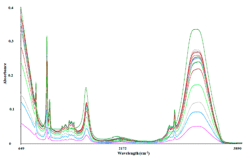
Datasets obtained from the FT-MIR spectroscopy were exported and transformed using Unscrambler software. The transformations applied (Figure 1) included: baseline offset, Multiplicative Scatter Correction (MSC), unit vector normalization, Savitzky-Golay smoothing with nine symmetry points, and finally the first (order one) and second (order two) derivatives of Savitzky-Golay with polynomial order two and six symmetry points.
In general, the elimination of baseline shifts helps to reveal hidden information and emphasize small spectral variations (Formosa et al., 2020). The MSC normalization was performed to correct each spectrum based on the mean value (average of all spectra) (Windig et al., 2008). The unit vector normalization and Savitzky-Golay smoothing were implemented to improve the signal by removing the noise of each spectrum (Haq et al., 2018; Wu et al., 2015).
Treatments 1 and 2 described in Figures 1 and 3 were evaluated and compared with the raw data using a multivariable approach, consisting of PCA, PLS-DA, and OPLS-DA routines. Figure 3 shows the plots of spectral data transformed by the first and second derivatives. Figure 3A, like Figure 3B, shows three regions, designed Region 1 from 1360 - 1766 cm-1, Region 2 from 1908 - 2172 cm-1, and Region 3 from 3361 - 3746 cm-1, indicating the difference between the data of both treatments 1 and 2. These differences could be reflected in the multivariate analysis.
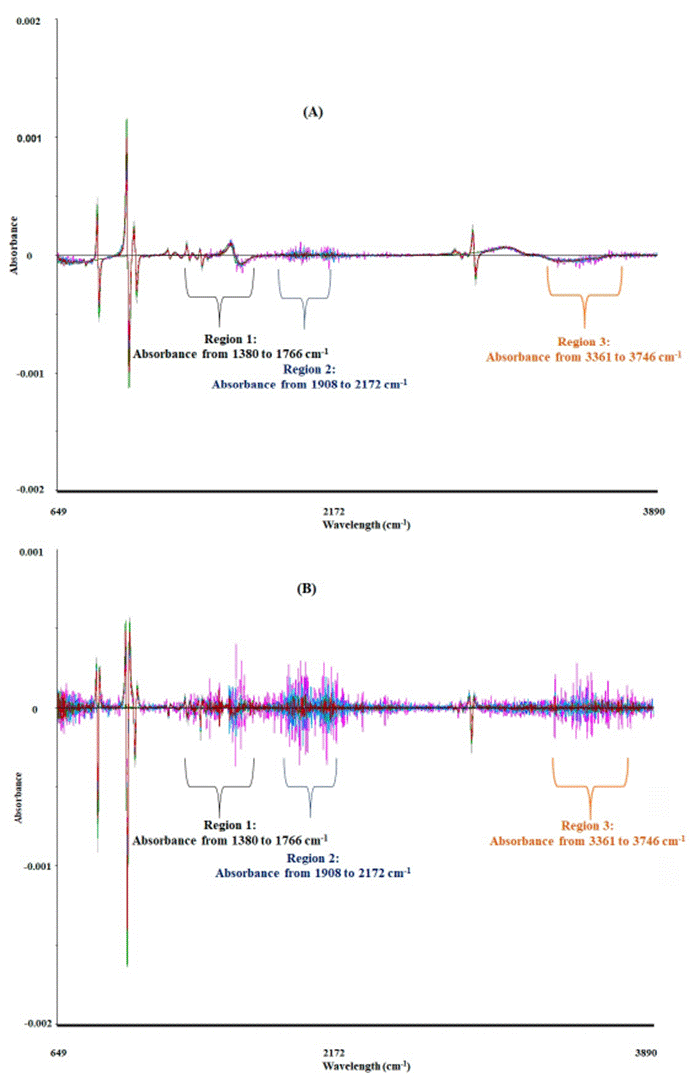
Figure 3 FT-MIR spectra of mezcales pretreated with the first (A) and second (B) derivative of Savitzky-Golay (polynomial order two and six symmetry points). Both data sets were transformed by baseline offset, multiplicative scatter correction, unit vector normalization, and Savitzky-Golay smoothing with nine symmetry points. This data matrix was subjected to multivariate analysis and its performance was evaluated.
Figura 3 Espectros de FT-MIR de mezcales pre-tratados con filtro Savitzky-Golay en primera derivada (A) y segunda derivada (B) (orden polinomial dos y seis puntos de simetria). Ambos conjuntos de datos fueron transformados con desplazamiento de linea base, correccion de dispersion multiplicativa, normalizacion de vectores unitarios y suavizado Savitzky-Golay con nueve puntos de simetria. Esta matriz de datos se sometio a analisis multivariado y se evaluo su desempeno.
Figure 4 shows the loadings plots based on PCA of the FT-MIR data matrix of mezcales produced with A. angustifolia, A. potatorum, A. salmiana, and A. karwinskii. Two principal components described 57.6 % of the spectral variation for FT-MIR raw data (Figure not shown); 51.3 % (treatment 1) and 27.9 % (treatment 2) for the pre-treated datasets (figures not shown). Although the spectral variation is greater for the FTMIR raw data, it is suspicious for two main reasons. The first reason is that a sample of mezcal elaborated with A. salmiana is located inside the ellipse of A. angustifolia, and the second reason is related to the advantage of analyzing a pre-treated matrix since the spectral transformation is necessary to minimize or eliminate physical effects. Specifically, a derivation procedure is applied to eliminate additive and multiplicative effects, and in addition, both transformations remove the baseline of the spectra (Anjos et al., 2016).
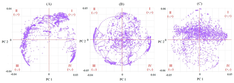
Additionally, the trends in Figure 4 correspond to the distribution of the loadings, which shows a homogeneity of the values in Figure 4(B and C), in contrast to Figure 4A. The distribution of the loadings around the four quadrants
(I, II, III, and IV) allows us to obtain reliable and robust models (López-Aguilar et al., 2021). A similar pattern is observed in the loadings of the PLS-DA model for species (Figure 5), Figure 5F shows better behavior and homogeneous data of transformed spectra with second derivative than raw spectra (Figure 5D) of the FT-MIR spectroscopy.
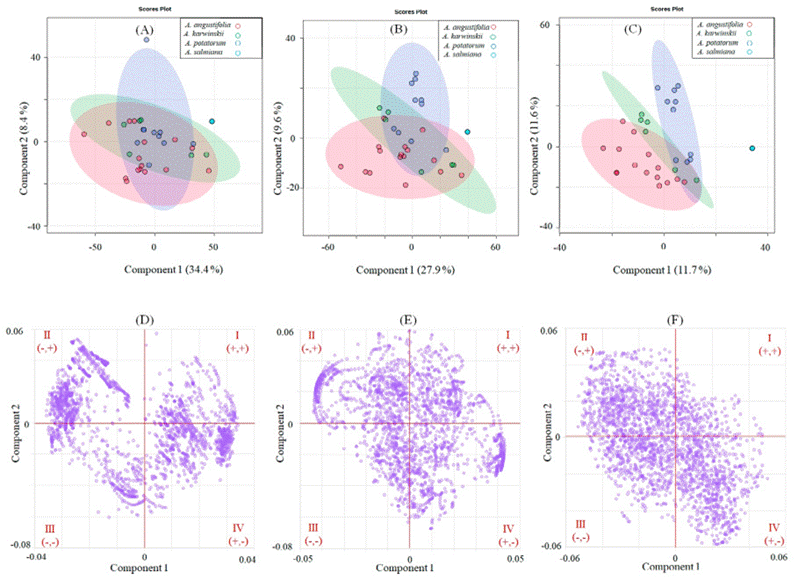
Figure 5 Partial Least Squares (PLS)-Discriminant Analysis (DA) of mezcales subjected to FT-MIR spectroscopy. The scores and loadings plots were performed on the raw [(A) and (D)], first derivative [(B) and (E)], and second derivative [(C) and (F)] data. The roman numerals indicate the quadrants of the graph (I, II, III, and IV).
Figura 5 Análisis Discriminante de Mínimos Cuadrados Parciales de mezcales sometidos a espectroscopía FT-MIR. Los gráficos de scores y de loadings se obtuvieron de los datos crudos [(A) and (D)], primera derivada [(B) and (E)], y segunda derivada [(C) and (F)]. Los números romanos indican los cuadrantes del gráfico (I, II, III, y IV).
However, the spectral variation represented by the scores plots in Figure 5C is only 23.3 % (component 1: 11.7 % and component 2: 11.6 %). Although the variation values are higher for the first derivative [Figure 5A; 42.8 % (component 1: 34.4 % and component 2: 8.4 %)] and raw data [Figure 5B; 37.5 % (component 1: 27.9 % and component 2: 9.6 %)], the scores plot shows a better separation for the second derivative data. The validation allowed us to evaluate the predictive power and accuracy (Ghosh et al., 2020) of the three models (raw spectra and transformed data with first and second derivatives) using leave one out-cross validation (LOO-CV) with 100 permutation routines and the value Q2 denotes the ability of the analysis (Westerhuis et al., 2008).
The results (Figure 6A) showed that the PLS-DA analysis derived from the raw spectra indicated low and negative Q2 values for the components, which means that the model is not prognostic at all or is overfitted (Szymańska et al., 2012). Furthermore, the observed p-value is not significant (Figure 6D; p = 0.8) by presenting 80 % of incorrect permutations, in contrast to other treatments, where the first and second derivative data had positive Q2 values for the five components [Figure 6(B and C) ] and the performance during the permutation tests was significant for the two models [Figure 6 (E and F)]. The permutation trials assume that there is no discrimination between the pair of randomly formed groups (Westerhuis et al., 2008).
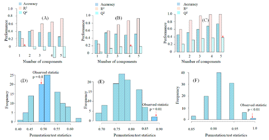
Figure 6 Performance of the Partial Least Squares (PLS)-Discriminant Analysis (DA) of mezcales subjected to FT-MIR spectroscopy. Q2 and p-value are based on the raw [(A) and (D), first derivative [(B) and (E)], and second derivative [(C) and (F)] data. The significance level of PLS-DA was set at 0.05.
Figura 6 Desempeño del Análisis Discriminante de Mínimos Cuadrados Parciales de mezcales sometidos a espectroscopía FT-MIR. Q2 y p-value se obtuvieron con base en los datos crudos [(A) y (D)], primera derivada [(B) y (E)], y segunda derivada [(C) y (F)]. La significancia del análisis OPLS-DA se estableció al 0.05.
Table 2 shows the capacity of the OPLS-DA on the FTMIR spectra according to applied transformation. The three pairwise comparisons from A. potatorum, A. angustifolia and A. salmiana [Figure 7(A, B, and C) ] made with raw data, presented Q2 values below 0.2 [Figure 8(A, B, and C)], in addition, the p-values showed no significant differences in the analysis (p ≥ 0.05). Apart from that, of the three comparisons made with data of the first derivative [Figure 7(D, E, and F) ], only the two comparisons between A. karwinskii and A. potatorum [Figure 7E], and A. angustifolia and A. karwinskii [Figure 7F], showed significance (p = 0.02) of the test for Q2 [Figure 8(E and F) ].
Table 2 Overview performance of the OPLS-DA model based on Q2 and p-value for the pairwise comparisons of A. potatorum, A. angustifolia, and A. karwinskii according to the applied transformation (first derivative or second derivative) on the FT-MIR spectral database.
Tabla 2 Resumen del desempeño del modelo OPLS-DA con base en Q2 y p-value para las comparaciones pareadas de A. potatorum, A. angustifolia, y A. karwinskii de acuerdo con la transformación aplicada (primera derivada o segunda derivada) sobre la base de datos espectral FT-MIR.
| Pretreatment | Statistical | A. angustifolia and A. potatorum | A. karwinskii and A. potatorum | A. angustifolia and A. karwinskii |
|---|---|---|---|---|
| Raw data | Q2 | -0.0858 | 0.134 | 0.149 |
| p-value | 0.22 | 0.11 | 0.06 | |
| First derivative | Q2 | 0.162 | 0.55 | 0.376 |
| p-value | 0.1 | 0.02 | 0.02 | |
| Second derivative | Q2 | 0.232 | 0.654 | 0.563 |
| p-value | 0.04 | < 0.01 | 0.01 |
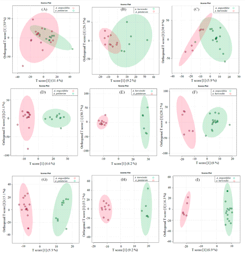
Figure 7 Score plots of mezcales subjected to FT-MIR spectroscopy and generated from Orthogonal Partial Least Squares (OPLS)-Discriminant Analysis (DA) on the raw [(A), (B), and (C)], first derivative [(D), (E), and (F)], and second derivative [(G), (H), and (I)] data. Pairwise comparisons were performed to evaluate the discriminations between A. angustifolia and A. potatorum [(A), (D), y (G)], A. karwinskii and A. potatorum [(B), (E), y (H)] , and A. angustifolia and A. karwinskii [(C), (F), y (I)].
Figura 7 Gráficos de score de mezcales sometidos a espectroscopía FT-MIR y generados del Análisis Discriminante mediante Mínimos Cuadrados Parciales Ortogonales sobre los datos crudos [(A), (B), y (C)], primera derivada [(D), (E), y (F)], y segunda derivada [(G), (H), y (I)]. Las comparaciones pareadas que se implementaron para evaluar discriminación fueron entre A. angustifolia y A. potatorum [(A), (D), y (G)], A. karwinskii y A. potatorum [(B), (E), y (H)], y A. angustifolia y A. karwinskii [(C), (F), y (I)].
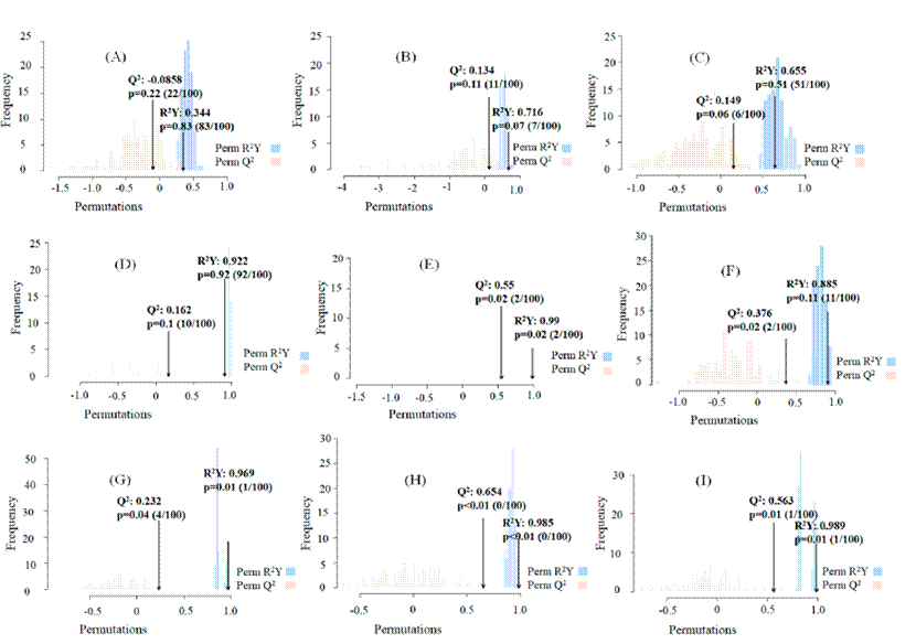
Figure 8 Orthogonal Partial Least Squares (OPLS)-Discriminant Analysis (DA) performance of the mezcales subjected to FT-MIR spectroscopy. R2Y, Q2, and p-value are based on the raw [(A), (B), and (C)], first derivative [(D), (E), and (F)], and second derivative [(G), (H), and (I)] data. Pairwise comparisons to evaluate the discriminations between A. angustifolia and A. potatorum [(A), (D), and (G)], A. karwinskii, and A. potatorum [(B), (E), and (H)], and A. angustifolia and A. karwinskii [(C), (F), and (I)] were performed. The significance of the OPLS-DA was set at 0.05.
Figura 8 Desempeño del Análisis Discriminante de Mínimos Cuadrados Parciales Ortogonales de mezcales sometidos a espectroscopía FT-MIR. R2Y, Q2, y p-value se obtuvieron con base en los datos crudos [(A), (B), y (C)], primera derivada [(D), (E), y (F)], y segunda derivada [(G), (H), y (I)]. Las comparaciones pareadas que se implementaron para evaluar discriminación fueron entre A. angustifolia y A. potatorum [(A), (D), y (G)], A. karwinskii y A. potatorum [(B), (E), y (H)], y A. angustifolia y A. karwinskii [(C), (F), y (I)]. La significancia del análisis OPLS-DA se estableció al 0.05.
The three pairwise comparisons between A. angustifolia, A. potatorum and A. karwinskii performed with the second derivative data matrix are also shown in Table 2 and Figure 7(G, H, and I). Interestingly, the three comparisons presented Q2 values statistically significant [Figure 8(G, H, and I)], for example, the comparison between A. angustifolia and A. potatorum [Figure 7G] had a Q2 value [Figure 8G] of 0.232 and a p-value of 0.04 (p < 0.05). Similarly, the discrimination between A. karwinskii and A. potatorum [Figure 7H] showed a Q2 value [Figure 8H] of 0.654 and a p-value less than 0.01 (p < 0.05). Finally, the discrimination between A. angustifolia and A. karwinskii [Figure 7I] showed a Q2 value [Figure 8I] of 0.563 and a p-value of 0.01.
Importantly, the lowest Q2 value was for the discrimination between A. angustifolia and A. potatorum [Figure 8G]. This suggests that of the three pairs of comparisons, it is more difficult to distinguish mezcales between these species, possibly because they are highly commercialized species and the agaves are mixed during the cooking step. Mezcal production includes more than 50 species of agave, of these, 22 are the most used, and A. angustifolia becomes important for presenting high yields (Castañeda-Nava et al., 2019; Sánchez-Gómez et al., 2022). Particularly, in localities from Sierra Sur, Oaxaca, the producers use 40 % of A. angustifolia and 15 % of A. potatorum of the total cultivated agave (Rios-Colín et al., 2022).
Determination of the ethanol percentage of mezcal based on FT-MIR spectroscopy
Training
The FT-MIR spectroscopy implemented in the 15 mezcales (Table 3) from 2021, allowed the calibration and validation of the ethanol percentage (% v/v) experimentally obtained by a PLS-R analysis, which is widely used for the construction of models that estimate the content of a compound of interest (Silva et al., 2014).
Table 3 FT-MIR spectroscopy data matrix of mezcales obtained in 2021, along with the corresponding experimental ethanol percentage (NMX-V013-NORMEX-2019), to generate a PLS-R model that allows the prediction of the ethanol percentage (% v/v).
Tabla 3 Matriz de datos de espectroscopía FT-MIR de mezcales obtenidos en 2021 junto con el correspondiente porcentaje de etanol experimental (NMX-V-013-NORMEX-2019) para generar un modelo PLS-R que permita la predicción del porcentaje de etanol (% v/v).
| Mezcal | Ethanolz | Absorbancey | ||||
|---|---|---|---|---|---|---|
| 1500.35x | 1500.83 | 1502.31 | …. | 1700.91 | ||
| 301 | 46.7 | 0.04 | 0.04 | 0.03 | 0.04 | |
| 310 | 41.9 | 0.04 | 0.04 | 0.04 | 0.05 | |
| 450 | 40.6 | 0.04 | 0.04 | 0.04 | 0.05 | |
| 470 | 46.0 | 0.03 | 0.03 | 0.03 | 0.04 | |
| 580 | 38.2 | 0.04 | 0.04 | 0.04 | 0.05 | |
| 601 | 48.2 | 0.03 | 0.03 | 0.03 | 0.03 | |
| 630 | 46.3 | 0.04 | 0.04 | 0.03 | 0.05 | |
| 640 | 46.8 | 0.04 | 0.04 | 0.04 | 0.04 | |
| 690 | 48.0 | 0.04 | 0.04 | 0.04 | 0.05 | |
| 701 | 48.2 | 0.03 | 0.03 | 0.03 | 0.04 | |
| 710 | 39.8 | 0.04 | 0.04 | 0.04 | 0.05 | |
| 790 | 47.1 | 0.04 | 0.04 | 0.04 | 0.05 | |
| 460 | 40.4 | 0.04 | 0.04 | 0.04 | 0.05 | |
| 760 | 45.0 | 0.04 | 0.04 | 0.04 | 0.05 | |
| 920 | 50.0 | 0.03 | 0.03 | 0.03 | 0.04 | |
z Experimental ethanol percentage (% v/v).
y Absorbance gained by FT-MIR spectroscopy of mezcales in 2021.
x Wavenumber (cm-1) that corresponds to the FT-MIR absorption region.
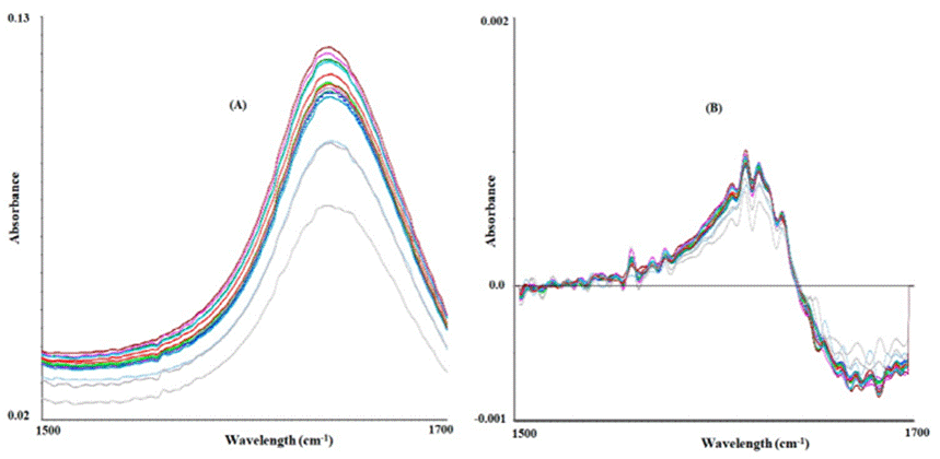
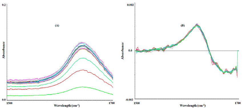
The MIR region used to calibrate and validate the ethanol percentage (% v/v), which in turn ranged from 1500 to 1700 cm-1 (Figure 9A), was subjected to a spectral transformation with the Savitzky-Golay first derivative of polynomial order two, and six symmetry points (Figure 9B). The infrared regions that have been evaluated were those corresponding to 1045 - 1086 cm-1 (Debebe et al., 2017) and three jointly evaluated regions comprising 663 - 1292, 1920 - 2236, and 2864 - 3057 cm-1 (Anjos et al., 2016), but no robust prediction models were found when these spectroscopic regions were evaluated in mezcal.
The R2 values in the calibration and validation of the PLS-R analysis were 0.98 and 0.81, respectively (Table 4). The RMSEC and RMSEP values were 0.41 and 1.68, which indicate the performance of the model with acceptable prediction values. Finally, the RPD ratios were 9.03 and 2.29, respectively. The behavior of the mezcal samples during calibration and validation is shown in Figure 10 and Table 5. It can also be seen that samples 601, 640 and 690, were distributed far from the rest of the samples during validation, which means that they were the ones that showed the highest variation between the estimated and the reference values (differences of 4.5, 2.1, and 2.6, respectively). Therefore, these three samples were the ones that contributed the most to the RMSEP values (1.68). It is important to highlight the good predictive capacity of samples 301 and 701, whose differences between the calibration and validation of the ethanol percentage were zero for both mezcales.
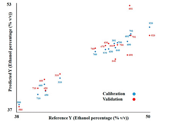
Table 5 Predicted ethanol percentage during the training of the PLS-R model based on the FT-MIR data matrix of the mezcales obtained in 2021.
Tabla 5 Porcentaje de etanol predictivo durante el entrenamiento del modelo PLS-R con base en la matriz de datos FT-MIR de los mezcales obtenidos en 2021.
| Mezcal | Reference Y1 | Predicted Y2 | Predicted Y3 | Difference1 | Difference2 |
|---|---|---|---|---|---|
| 301 | 46.8 | 47.1 | 46.8 | 0.3 | 0 |
| 310 | 41.9 | 42 | 42.6 | 0.1 | 0.7 |
| 450 | 40.6 | 40.1 | 40.2 | 0.5 | 0.4 |
| 470 | 46 | 46.2 | 46.8 | 0.2 | 0.8 |
| 580 | 38.2 | 38.1 | 37.8 | 0.1 | 0.4 |
| 601 | 48.2 | 48.3 | 52.7 | 0.1 | 4.5 |
| 630 | 46.3 | 46.3 | 47.1 | 0 | 0.8 |
| 640 | 46.9 | 46.5 | 44.8 | 0.4 | 2.1 |
| 690 | 48 | 47.4 | 45.4 | 0.6 | 2.6 |
| 701 | 48.3 | 48.5 | 48.3 | 0.2 | 0 |
| 710 | 39.9 | 39.6 | 40.5 | 0.3 | 0.6 |
| 790 | 47.1 | 47.2 | 46.9 | 0.1 | 0.2 |
| 460 | 40.5 | 41.1 | 41.8 | 0.6 | 1.3 |
| 760 | 45.1 | 45.9 | 46.4 | 0.8 | 1.3 |
| 920 | 50 | 49.5 | 48.3 | 0.5 | 1.7 |
Reference Y1: indicates the experimental ethanol percentage (reported as % v/v).
Predicted Y2: the ethanol percentage gained during the calibration of the PLS-R model (reported as % v/v).
Predicted Y3: the ethanol percentage gained during the validation of the PLS-R model (reported as % v/v).
Difference1 = absolute value of the subtraction of the Predicted Y2 from Reference Y1.
Difference2 = absolute value of the subtraction of the Predicted Y3 from Reference Y1.
Testing
The PLS-R model applied to the FT-MIR data matrix of the mezcales analyzed in 2021, was used to predict the ethanol percentage (% v/v) of a set of samples obtained in 2022 (Table 6) and subjected to FT-MIR analysis. The region evaluated during testing (Figure 11A) was the same as that used during training (1500-1700 cm-1), which was also subjected to a spectral transformation with the Savitzky-Golay first derivative of polynomial order two, and six symmetry points (Figure 11B).
Table 6 Data matrix of the FT-MIR spectroscopy, performed in mezcales obtained in 2022, along with the corresponding experimental ethanol percentage (NMX-V-013-NORMEX-2019) to generate a PLS-R model that allows the prediction of the ethanol percentage (% v/v).
Tabla 6 Matriz de datos de la espectroscopía FT-MIR realizada en mezcales obtenidos en 2022 junto con el correspondiente porcentaje de etanol experimental (NMX-V-013-NORMEX-2019) para generar un modelo PLS-R que permita la predicción del porcentaje de etanol (% v/v).
| Mezcal | Ethanolz | Absorbancey | ||||
|---|---|---|---|---|---|---|
| 1500.35x | 1500.83 | 1502.28 | …. | 1700.91/0.05 | ||
| 239-1 | 47.0 | 0.04 | 0.04 | 0.04 | 0.05 | |
| 239-2 | 47.1 | 0.04 | 0.04 | 0.04 | 0.05 | |
| 239-3 | 47.4 | 0.04 | 0.04 | 0.04 | 0.05 | |
| 245-1 | 46.2 | 0.04 | 0.04 | 0.04 | 0.05 | |
| 245-2 | 46.6 | 0.04 | 0.04 | 0.04 | 0.05 | |
| 245-3 | 46.6 | 0.04 | 0.04 | 0.04 | 0.04 | |
| 373-1 | 49.3 | 0.04 | 0.04 | 0.04 | 0.05 | |
| 373-2 | 49.2 | 0.04 | 0.04 | 0.04 | 0.05 | |
| 373-3 | 49.4 | 0.01 | 0.01 | 0.01 | 0.01 | |
| 688-1 | 49.4 | 0.04 | 0.04 | 0.04 | 0.05 | |
| 688-2 | 49.4 | 0.04 | 0.04 | 0.04 | 0.04 | |
| 688-3 | 49.4 | 0.04 | 0.04 | 0.03 | 0.04 | |
| 863-1 | 39.9 | 0.04 | 0.04 | 0.04 | 0.05 | |
| 863-2 | 39.6 | 0.02 | 0.02 | 0.02 | 0.03 | |
| 863-3 | 40.0 | 0.04 | 0.04 | 0.04 | 0.05 | |
| 949-1 | 48.9 | 0.03 | 0.03 | 0.03 | 0.04 | |
| 949-2 | 49.1 | 0.04 | 0.04 | 0.04 | 0.04 | |
| 949-3 | 49.3 | 0.03 | 0.03 | 0.03 | 0.04 | |
z Experimental ethanol percentage (% v/v).
y Absorbance gained by FT-MIR spectroscopy of mezcales in 2022.
x Wavenumber (cm-1) that corresponds to the FT-MIR absorption region.
The prediction of the ethanol percentage (% v/v) for the new set of samples obtained in 2022 (Table 7) and subjected to FT-MIR analysis in triplicate, based on the PLS-R model performed with the samples evaluated in 2021, allowed us to obtain the ethanol percentage in an approximate way. For example, samples 373-1 and 688-1 showed the highest difference between the reference value and predicted value (8.3 y 5.8 %), but it is also important to highlight that samples 245-1 and 863-3 showed the lowest difference value (0.6 and 0.7 %, respectively). As a result, the RMSEP and R2 values were 2.32 and 0.55, respectively, which showed an opposite behavior to that obtained in training, since the RMSP was greater and the R2 was lower. Moreover, the RPD was 1.27 which is lower than the value obtained in the validation (2.29); since the RPD indicates the predictability of a model (Kamruzzaman, 2021), then high RPD values are required.
Table 7 Predicted ethanol percentage (% v/v) at the testing step of the PLS-R model based on the FT-MIR data matrix of the mezcales obtained in 2022.
Tabla 7 Porcentaje de etanol (% v/v) predictivo en la etapa de prueba, del modelo PLS-R con base en la matriz de datos FT-MIR de los mezcales obtenidos en 2022.
| Mezcal | Reference Y | Predicted Y | Difference |
|---|---|---|---|
| 239-1 | 47 | 44.6 | 2.4 |
| 239-2 | 47.1 | 44.4 | 2.7 |
| 239-3 | 47.4 | 44.4 | 3.0 |
| 245-1 | 46.2 | 46.8 | 0.6 |
| 245-2 | 46.6 | 44.5 | 2.1 |
| 245-3 | 46.6 | 48.1 | 1.5 |
| 373-1 | 49.3 | 41.0 | 8.3 |
| 373-2 | 49.2 | 46.6 | 2.6 |
| 373-3 | 49.4 | 47.3 | 2.1 |
| 688-1 | 49.4 | 43.6 | 5.8 |
| 688-2 | 49.4 | 46.7 | 2.7 |
| 688-3 | 49.4 | 48.4 | 1.0 |
| 863-1 | 39.9 | 40.9 | 1.0 |
| 863-2 | 39.6 | 38.4 | 1.2 |
| 863-3 | 40.0 | 39.3 | 0.7 |
| 949-1 | 48.9 | 46.6 | 2.3 |
| 949-2 | 49.1 | 45.3 | 3.8 |
| 949-3 | 49.3 | 46.1 | 3.2 |
Reference Y: indicates the experimental ethanol percentage (reported as % v/v).
Predicted Y: the ethanol percentage gained during the prediction based on the PLS-R model performed with samples obtained in 2021 (reported as % v/v).
Difference = absolute value of the subtraction of Predicted Y from Reference Y.
Despite the behavior observed in the prediction (three samples presented the highest dissimilarity between the estimated and the reference value), this proposal can be the basis for determining the ethanol percentage (% v/v) by FT-MIR. This technique is a simple, fast, accurate, reliable, and viable alternative compared to traditional methods such as GC or densitometry which are more laborious (Debebe et al., 2017; Quintero-Arenas et al., 2020).
Conclusions
The PLS-DA with transformed data by both first (p = 0.01) and second (p < 0.01) derivatives, allowed the differentiation of mezcales produced from Agave angustifolia, Agave potatorum, Agave salmiana, and Agave karwinskii, while OPLS-DA was more robust when analyzed with second-derivative data. Pairwise comparisons by OPLS-DA, allowed us to discriminate the mezcales between A. angustifolia and A. potatorum (Q2 = 0.232, p-value = 0.04; R2Y = 0.969, p-value = 0.01), A. karwinskii and A. potatorum (Q2 = 0.654, p-value < 0.01; R2Y = 0.985, p-value < 0.01), and A. angustifolia and A. karwinskii (Q2 = 0.563, p-value = 0.01; R2Y = 0.989, p-value = 0.01). The FT-MIR and multivariate analysis allowed the prediction of the ethanol percentage (% v/v) of the mezcales obtained in 2022, based on the PLS-R model previously run on the samples evaluated in 2021. During training, the R2 values in the calibration and validation of the PLS-R analysis were 0.98 and 0.81, respectively. The RMSEC and RMSEP coefficients were 0.41 and 1.68, respectively. However, in testing, the behavior was the opposite, since the R2 value (0.55) was lower and the RMSEP was higher (2.08). Finally, although we declare that the capacity of the PLS-R model was acceptable, it can be the basis for generating new ones, as more samples will be analyzed.


 nueva página del texto (beta)


