


 nueva página del texto (beta)
 Inglés (pdf)
 Artículo en XML
 Referencias del artículo
 Enviar artículo por email
 Citado por SciELO
  Similares en
SciELO
Similares en
SciELO 
 Permalink
Introduction
Natural ventilation (NV) in buildings can cut fan and cooling energy use, improving indoor air quality and occupant comfort during hot seasons. Architects and engineers increasingly rely on thermal building simulations for design and retrofitting, making accurate NV simulations crucial.
Building thermal and energy performance simulation encompasses physical models, statistical techniques, and hybrid models (Foucquier et al., 2013). Physical models analyze the thermal and energy performance of a specific building. Statistical methods assess energy performance for specific building types in particular areas. Physical models are further categorized into computational fluid dynamics (CFD), zonal, and multizone (nodal) approaches. CFD provides three-dimensional air temperature and velocity insights but is time-intensive for year-long whole-building simulations. Zonal modeling offers two-dimensional air temperature and velocity data and suits large space buildings (Lu et al., 2020). Multizone (nodal) modeling treats each building zone as a uniform entity, making it suitable for year-long whole-building simulations.
Multizone building thermal and energy simulation software, like EnergyPlus (EP), incorporates the multizone Airflow Network model (AFN) to simulate natural or mechanical ventilation (ASHRAE, 2013). AFN comprises interconnected nodes and airflow components, where node variables represent pressure and linkage variables denote airflow rates. AFN of EP (EP-AFN) operates through three sequential stages: pressure and airflow computations, node temperature and humidity evaluations, and sensible and latent load assessments (DOE, 2016). EP offers two additional ventilation models alongside the AFN: the Design Flow Rate and the Wind and Stack Open Area models (DOE, 2016). The first model may not replicate realistic conditions for NV since it relies on a predetermined flow rate. The second model is tailored for NV but has a notable drawback. It calculates the flow rate based on wind speed, thermal buoyancy, area, and the discharge coefficient (Cd) of the opening, without considering the presence of other openings in the thermal zone. This omission can lead to inaccuracies in results.
EP provides various room air models, with the Cross Ventilation model being the only one that furnishes air velocity data for three distinct regions within the thermal zone (the jet, recirculation, and window jet).
In EP-AFN, input parameters include the wind pressure coefficient (Cp) for each external node and the discharge coefficient (Cd) for each opening. Additionally, the opening factor, representing the fraction of the opening allowing airflow, must be specified for each opening (DOE, 2016).
There are several studies that report EP simulations using natural, mechanical, or mixed-mode ventilation, but relatively few of them explicitly report the use of the AFN.
EP-AFN has been applied to mechanically ventilated buildings (Rusly & Piechowski, 2011; Yan et al., 2015; Cheng et al., 2017), to double skin facades of air-conditioned buildings (Chan et al., 2009; Hashemi et al., 2010; Choi et al., 2012; Joe et al., 2013; Sung et al., 2013; Le et al., 2014; Peng et al., 2016; Andelković et al., 2016), and to air-conditioned buildings that employ natural night ventilation for energy saving purpose (Ramponi et al., 2014; Albuquerque et al., 2020).
EP-AFN has also been applied in naturally ventilated buildings (Zhai et al., 2011; Zhang et al., 2013; Schulze & Eicker, 2013; Belleri et al., 2014; Arendt et al., 2017; Gimenez et al., 2018; Shirzadi et al., 2018; Dogan & Kastner, 2021; Goncalves et al., 2022, Chu, 2023; Li & Chen, 2023; Salvati & Kolokotroni, 2023; Yin & Muhieldeen, 2024). Most of these studies assessed the accuracy of EP-AFN in specific building context (Zhai et al., 2011; Zhang et al., 2013; Belleri et al., 2014; Arendt et al.,2017; Gimenez et al., 2018; Goncalves et al., 2022; Li & Chen, 2023; Chu, 2023; Salvati & Kolokotroni, 2023; Yin & Muhieldeen, 2024). Other studies considered generic cross-ventilation cases solely with the wind effect (Shirzadi et al., 2018; Chu, 2023). Other authors studied the impact of the wind pressure coefficient on the ventilation building (Xie et al., 2023; Sakiyama et al., 2024). Some investigations compared simulation outcomes to field measurements (Zhai et al., 2011; Belleri et al., 2014; Arendt et al., 2017; Shirzadi et al., 2018), focusing on parameters like the indoor air temperature (T i ) (Zhai et al., 2011; Belleri et al., 2014; Arendt et al., 2017) and the ventilation flow rate (Q) (Zhang et al., 2013; Belleri et al., 2014; Arendt et al., 2017; Shirzadi et al., 2018). Also, the air changes per hour (ACH) and the annual cooling degree hours have been employed as parameters (Gimenez et al., 2018). Certain studies enhance accuracy by coupling EP (Zhang et al., 2013; Goncalves et al., 2022) or other multi-zone programs (Tan & Glicksman, 2005; Ohba & Lun, 2010) with CFD simulations, though this approach may pose challenges in buildings with numerous zones. A gap exists in assessing the accuracy of models in EP-AFN for generic naturally ventilated buildings that incorporate both wind and buoyancy effects. This study aims to address this gap by evaluating the precision of EP-AFN simulations through a comparison with CFD simulations. Specifically, it examines two natural ventilation configurations: cross ventilation and upward cross ventilation, within a generic isolated building. The analysis accounts for wind and buoyancy effects, with variations in wind speed and heating. Two heating modes are considered: internal heat gains and floor temperature.
In this study, CFD simulations serve as a reference for evaluating EP-AFN results. To ensure the credibility of CFD simulations, they have undergone validation against experimental data. In the literature, numerous studies validate CFD simulations for natural ventilation cases, primarily focusing on wind effects. Some examples of these validations are (Castillo & Huelsz, 2017; Kobayashi et al., 2022; Kumar et al., 2021; Zheng et al., 2020; Castillo et al., 2019; Kosutova et al., 2019; van Hooff et al., 2017; van Hooff & Blocken, 2010; Peren et al., 2015; Perén et al., 2015; Ramponi & Blocken, 2012). However, there are fewer reports validating CFD simulations for cases involving thermal buoyancy effects (Kosutova et al., 2018; Gilani et al., 2016). The CFD simulations presented in this paper are validated with experimental studies that consider the wind effect (Kurabuchi et al., 2004; Cruz-Salas et al., 2014) and another one that considers both effects (Lishman & Woods, 2006).
Study cases
The natural ventilation, in steady state, of a generic isolated building is considered. The fixed parameters for all cases are: outdoor air temperature and relative humidity, atmospheric pressure, wind profile and direction, and no radiative heat exchanges. The walls and roofs are considered adiabatic. The fact of neglecting the solar radiation effect makes the case more generic. The consideration of adiabatic walls and roofs increases the ventilation effect, which is the purpose of the present study, and this condition is close to the highly insulated envelopes.
Two configurations are analyzed: cross ventilation (CV) and upward cross ventilation (UCV). In the CV configuration, the building has two axial opposite windows at the center of the wall, one at windward and the other one at leeward. In the UCV the building has a window at windward and one windexchanger (WE) (Cruz-Salas et al., 2014; Castillo et al., 2017) on the roof with a single opening at leeward. Thus, the WE opening is at a higher level than that of the window.
Building geometries for both configurations are shown in Figure 1. In the CV configuration, the building has an internal area of 4.20 m×4.20 m and an internal height of 2.10 m, with two opposite windows of 0.90 m×0.45 m. The building roof is flat. This geometry was taken from (Kurabuchi et al., 2004). In the UCV configuration, the building has an internal area of 3.0 m×3.0 m and an internal height of 2.7 m. The window is square with a side length of 1.30 m, it is horizontally centered on the wall and its base is at 0.90 m from the floor. The WE is at the center of the building roof, it has a square cross-section duct with an internal side length of 0.65 m, and an internal height of 1.40 m when measured from the rooftop. The WE has a single square opening area equal to that of the WE duct cross-section. The building and the WE roof are flat. This building geometry was taken from the C0LW case of (Castillo et al., 2017).
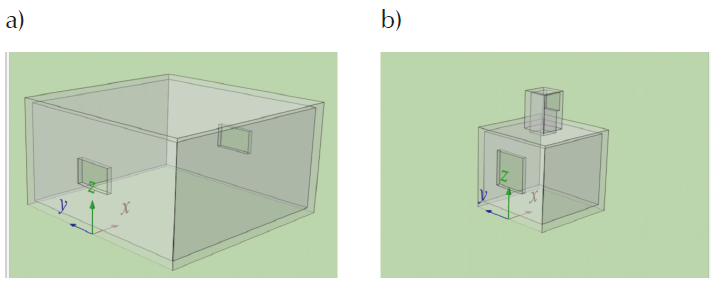
Figure 1 Building geometry for both configurations: a) cross ventilation (CV) and b) upward cross ventilation (UCV)
Two heating modes are considered for the CV and UCV configurations. Each one of these has four heating levels. One mode sets the rate of heat flow through the floor (q) (H cases), with values: 0 W, 250 W, 500 W and 750 W. The other mode sets the floor temperature (T cases), with values: 15°C, 25°C, 35°C and 45°C. Therefore, there are four groups of cases: CV-H, UCV-H, CV-T and UCV-T. Additionally, the wind speed at a 10 m height (ν10) varies along five values: 0.1 m/s, 0.5 m/s, 1 m/s, 3 m/s, and 5 m/s. Thus, a total of 80 study cases are tested.
CFD simulations
Three dimensional simulations are performed with the commercial CFD code ANSYS Fluent 19 (ANSYS, 2018).
General settings and parameters
For all simulations, the grids are generated with the surface cell extrusion
technique, obtaining a block structured grid with hexahedral cells (van Hooff & Blocken, 2010). The height
of the first cell extrusion z1 = 2.1
ks = 0.002 m is calculated according to Castillo et al. (2019). A
grid growing factor of 20 % is used. The domain dimensions are set according to
the guidelines given by Franke et
al. (2007) and Tominaga
et al. (2008). Three grids are generated for the
grid sensitivity analysis. The course grid and the fine grid are built
multiplying each spatial coordinate of the base grid by (1/2)1/3 and
21/3, respectively. The steady RANS equations are solved with the
SIMPLEC algorithm for pressure and velocity coupling using a second order upwind
scheme. Second order discretization schemes are used for the convection and the
viscous terms of the governing equations (Ramponi & Blocken, 2012). 10,000 iterations are set as the
stopping criteria. Convergence is considered to have been reached if the scaled
residuals are less than 10−5. The inlet boundary condition for the
velocity profile is the logarithmic law
Validation of wind-driven cross ventilation
Experimental results of a wind-driven CV case (Figure 2a, b) obtained in a wind tunnel using particle image velocimetry (PIV) by Kurabuchi et al. (2004) are used for the CFD validation. This validation has been presented in detail by the authors in (Castillo & Huelsz, 2017).
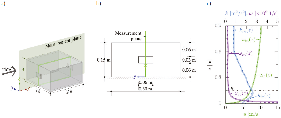
Figure 2 Wind driven cross ventilation case for validation: a) scaled model isometric view with measurement plane, b) scaled model front view with dimensions and c) vertical profiles of the air velocity, u; turbulent kinetic energy, k, and the specific dissipation rate, ω, at the inlet (solid line) and at the incident position (dashed line) in the empty domain. The subscripts in and ic refer to inlet and incident, respectively. Data from Kurabuchi et al. (2004)
In the CFD simulations, the values of
Figure 3a shows a small grid sensitivity
along the center line Lr (base grid has 1,448,712 cells). The average
difference of the
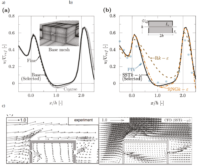
Figure 3 Wind driven cross ventilation case for validation: a) grid
sensitivity analysis comparing the normalized air velocity
Validation of wind driven upward cross ventilation
Experimental results of a wind driven UCV case (Figure 4a, b) obtained using an open water channel (OWC) and stereoscopic particle image velocimetry (SPIV) (Cruz-Salas et al., 2014) are used for the CFD validation. The validation was performed following the methodology in (Castillo et al., 2019), because the UCV case is similar to the case validated in that work.
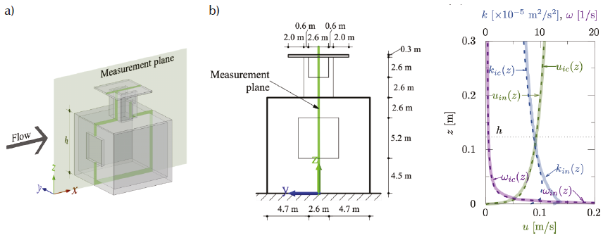
Figure 4 Wind driven upward cross ventilation case for validation: a) scaled model isometric view with measurement plane, b) scale model front view with dimensions, and c) vertical profiles of the fluid velocity, u; turbulent kinetic energy, k, and the specific dissipation rate, ω, at the inlet (solid line) and at the incident position (dashed line) in the empty domain. The subscripts in and ic refer to inlet and incident, respectively
In the CFD simulation, the computational domain (base grid with 1,837,108 cells)
is constructed to reproduce the OWC test section. This domain has a deviation
from the guidelines (Franke et
al., 2007; Tominaga
et al., 2008), but it is required in order to
reproduce the narrow width of the OWC. The values of
In Figure 5a,
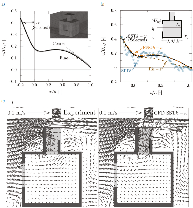
Figure 5 Wind driven upward cross ventilation case for validation: a) grid
sensitivity analysis comparing the normalized air velocity
Validation of wind and buoyancy driven upward cross ventilation
Experimental results of a case with the UCV configuration considering wind and buoyancy effects reported in (Lishman & Woods, 2006) are used for the CFD validation. The experiments employed water in a flume and thermocouple measurements (Figure 6a, b). The validity of the ventilation experiments using water is given in terms of the fact that the laboratory model and the real building have geometric, kinematic, and dynamic similarity. This validation is presented in more detail than the previous ones since it is the first time it is being reported. Lishman & Woods (2006) used a scaled model of a building with circular openings, 7 at the top in the windward facade and 7 at the bottom in the leeward facade. The flume had a transversal section area of 0.5 m × 0.5 m. The heat was supplied from the model floor by a heating plate with a series of high resistance metal coils. Five values of the heat flow rate q were tested (0 W, 11 W, 42 W, 76 W, 120 W). The temperature was measured using 4 thermocouples vertically distributed within the interior of the model. The thermocouples had an uncertainty of ±0.1.
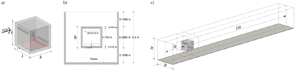
Figure 6 Scaled model of a building with circular top openings at its windward facade and bottom openings at its leeward facade: a) right isometric view, b) front view with dimensions and c) isometric view of the computational domain with dimensions. h = 0.2085 m is the characteristic length
For the CFD simulations, the physical properties of the fluid are obtained from (Lishman & Woods, 2006). The Boussinesq approximation is used. In the convergence criteria the scaled residuals for energy are equal to 10−7. The computational domain is constructed to reproduce the flume test section (Figure 6c). This domain also has a deviation from the guidelines (Franke et al., 2007; Tominaga et al., 2008). Three grids with hexahedral cells are generated (Figure 7a): the coarse grid has 270,079 cells; the base grid has 576,628 cells and the fine grid has 1,074,406 cells. Constant values of u and the turbulence intensity are set at the domain inlet (0.01 m/s and 0.1, respectively). Free slip condition (Gallardo et al., 2013) is set at the domain top. The lateral walls of the domain are specified as smooth no slip walls. q is applied as a constant heat flux on the building floor. In Figure 7a the streamwise gradients of the u, k and ω profiles are presented. Their values are smaller than 6 %.
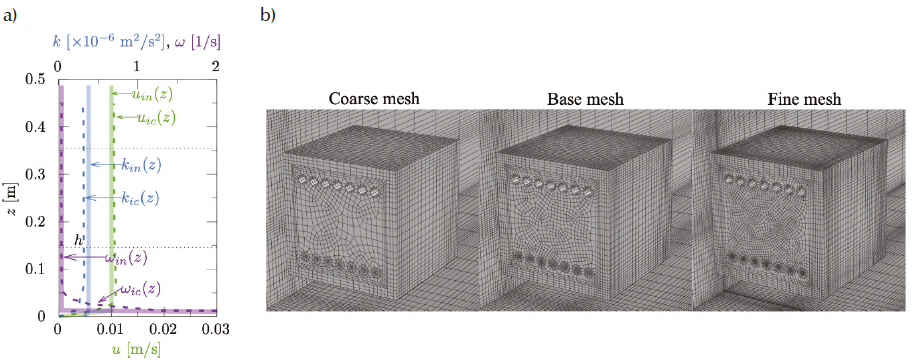
Figure 7 Wind and buoyancy driven upward cross ventilation case for CFD validation: a) streamwise gradients of the fluid x-component velocity, u, the turbulent kinetic energy, k, and the specific dissipation rate, ω, at the inlet (solid line) and at the incident position (dashed line) in the empty domain. The subscripts in and ic refer to inlet and incident, respectively. And b) isometric view of three grids of the model: coarse, base and fine
In Figure 8
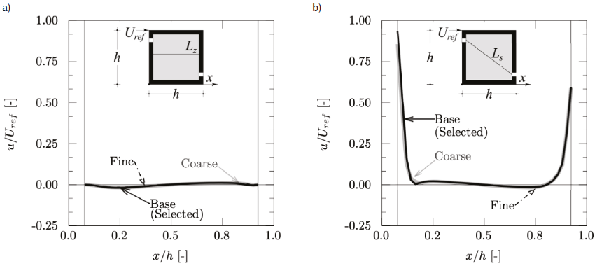
Figure 8 Grid sensitivity analysis of the normalized air velocity
The temperature difference between the indoor and outdoor fluid ∆T from three turbulence models (SST k−ω, R k−ε and RNG k−ε) is compared to the experimental results from (Lishman & Woods, 2006). The results for different values of q are shown in Table 1. For all values of q, the average of the absolute difference of ∆T between the turbulence model and the experiment is 0.3oC for SST k−ω and RNG k−ε, while for R k−ε is 0.4oC. Therefore, the three turbulence models are suitable for this UCV case. The SST k−ω model is selected for further simulations because this turbulence model is also accurate in the CV and UCV cases that only consider wind effect. Thus, the simulations of the UCV configuration with wind and buoyancy effects are validated. The parameters and settings of this section are applied to the simulation reported in the Results and discussion section.
Table 1 Heat flow rate q and temperature absolute difference between the indoor and outdoor fluids ∆T. The data are obtained from experiments (Lishman & Woods, 2006) and from CFD simulations with three different turbulence models: SST k−ω, RNG k−ε and R k−ε
| q [W] | ∆T [o C] | |||
|---|---|---|---|---|
| Experiment | SST k−ω | RNG k−ε | R k−ε | |
| 11 | 0.1 | 0.4 | 0.4 | 0.6 |
| 42 | 0.4 | 0.8 | 0.7 | 1.0 |
| 76 | 0.9 | 1.1 | 1.0 | 1.3 |
| 120 | 1.7 | 1.3 | 1.3 | 1.6 |
Obtaining opening coefficients
The pressure coefficient Cp is a dimensionless parameter that is the difference between the local pressure and the reference pressure divided by the reference dynamic pressure, given by
where p [Pa] is the local pressure, pref [Pa] is the static pressure in the freestream, ρref [kg/m3] is the freestream fluid density and uref is a reference velocity. EP uses the freestream velocity at the midheight of the opening as the reference velocity.
In the CFD simulations the value of Cp for an opening is obtained with the area weighted average (ANSYS, 2018).
The airflow rate Q [m3/s] is calculated as the total inflow through all openings.
The discharge coefficient Cd is a characteristic parameter of an opening. It is the result of the contraction and friction of the flow and depends on the opening geometry (Karava et al., 2004). For each opening functioning as entrance, Cd is calculated using:
where Qj is the inflow and Aj the area of the opening.
EnergyPlus simulations settings
The geometry of each configuration is modeled with Sketchup 2017. A single thermal zone is considered for both configurations. In order to simulate the walls and roofs as adiabatic, they are considered as being made from 15 cm thick expanded polystyrene with the Outside Boundary Condition set as Adiabatic. In EP an opening cannot be defined within an adiabatic surface. Therefore, for any wall with an opening, a 5 cm wide frame around the opening is considered. The Outside Boundary Condition of this frame is set as Outdoors. Constructions thermal absorptance and the ground reflectance are set equal to 0.0001 in order to simulate a nonradiative heat exchange condition.
For the H cases the heat flux through the floor is set using ZoneHVACRadiant:Electric. Additional simulations are performed using the same heat flux while considering that the heat flux is produced by people (sensible heat). The results are the same for both types of heat sources. For T cases, the floor is set as Ground and it is considered to be made of steel with a thickness of 0.001 m.
To create a steady state, the object SizingPeriod:DesignDay can be used (Schulze & Eicker 2013). This can also be achieved by modifying the weather file. In this study, the latter procedure is employed. Five weather files, one for each wind speed value, are created using the Weather Statistics and Conversions of EP. Each weather file has constant values for all variables. In all files, the outdoor air temperature To = 15°C, the atmospheric pressure is 1 atm, the relative humidity is 11 % (this is used to achieve the same air density considered in the CFD simulations), the solar radiation is zero and the wind direction is 0°. In EP, the radiative heat exchange to the sky is eliminated by setting the sky temperature as equal to To. The atmospheric boundary layer considered is that of a semi-urban area with a wind speed profile exponent of 0.25 and a 395 m thickness. The value of To is considered to be independent from the height.
The conduction transfer function algorithm is used. Since the simulations are in steady state, both the use of the input object Material:NoMass and that of the input object Material produce the same results. The Cross Ventilation model is used as the room air model. This model distinguishes two types of regions inside the building: main jet and recirculation. EP assesses whether the cross-ventilation model applies or not. If it does, EP uses this model, if it does not, EP uses the Mixing model. The TARP algorithm was used to model internal convection because it showed the best results in (Zhang et al., 2013).
The simulations are made using two groups of coefficients in EP-AFN. In the first group (C1), the discharge coefficient for openings at windward is set equal to the value often assumed in the literature for a large opening functioning as an entrance (Cd−lit = 0.6) (Heiselberg et al., 2001). The pressure coefficient is set equal the one calculated by EP (Cp−EP) for each wall and roof of the building as a function of wind direction, building height, and footprint aspect ratio. In the second group (C2), the coefficients are obtained from the CFD simulations (Cd−CFD, Cp−CFD), as described in the section obtaining opening coefficients. The values for these coefficients are shown in Table 2. The existence of Cp > 1.0 values is due to the fact that the Cp obtained from CFD simulations are calculated in accordance to the EP consideration, i.e the use of freestream velocity at midheight of the opening as the reference velocity. In EP the maximum value of Cp accepted for windward openings is 1. Therefore, the input values of Cp−CFD used in EP were set by EP as 1. For C1 and C2, the value of Cd is set as 1.0 (Linden et al., 1990) for all leeward openings. All openings are set as Detailed Opening. It was found that the use of the Simple Opening type produces errors when the temperature difference in the zone is zero. The airflow rate, Q [m3/s], is calculated as the sum of the inlet flow through all openings.
Table 2 Coefficients considered in C1 and C2. Discharge coefficients and pressure coefficients for openings at windward (ww) and leeward (lw), for the two configurations and for the wind speed at a 10 m height (v10)
| v10 | C1 | C2 | |||||
| Configuration | [m/s] | Cd-lit [-] | Cp-EP [-] | Cd-CFD [-] | Cp-CFD [-] | ||
| ww | ww | lw | ww | ww | lw | ||
| CV | 0.1 | 0.60 | 0.60 | -0.36 | 0.51 | 1.21 | -0.22 |
| 0.5 | 0.60 | 0.60 | -0.36 | 0.52 | 1.24 | -0.20 | |
| ≥1 | 0.60 | 0.60 | -0.36 | 0.52 | 1.04 | -0.17 | |
| UCV | 0.1 | 0.60 | 0.60 | -0.36 | 0.16 | 1.22 | -0.37 |
| 0.5 | 0.60 | 0.60 | -0.36 | 0.16 | 1.22 | -0.34 | |
| ≥1 | 0.60 | 0.60 | -0.36 | 0.15 | 1.13 | -0.43 | |
Results and discussion
Figure 9 shows temperature contour plots at the vertical central plane and on the floor for the CV and UCV configurations. These results are obtained for T cases with v10 = 0.01 m/s and a floor temperature of 45°C. For both configurations the highest indoor air temperature is close to the floor, forming a ring. As expected, the lowest temperature is at the incoming jet from the windward window. For the CV configuration, the temperature is around 27°C at the central vertical plane. The same temperature is found at the central zone close to the floor. For the UCV configuration, the temperature is around 17oC at the central vertical plane and around 22°C at the central zone close to the floor. The average indoor air temperatures of the CV and UCV are 27°C and 19oC, respectively.
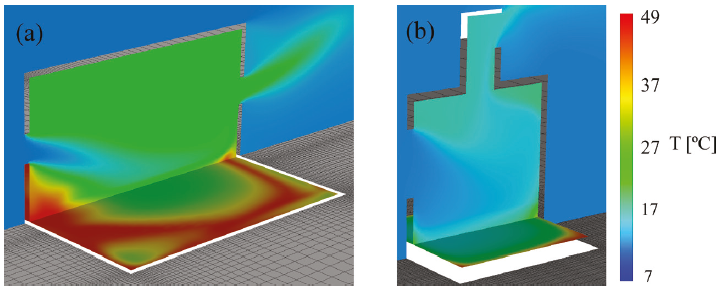
Figure 9 Temperature contour plots at the vertical central plane and on the floor, for T cases with v10 = 0.01 m/s and floor temperature of 45°C, a) cross ventilation and b) upward cross ventilation configurations
Results of the EP simulations using the coefficient groups C1 and C2 are compared with the results from the CFD simulations. Two comparison parameters are used: ∆T and Q.
Due to the configuration of the cases, the cross-ventilation model is set as the room air model for all cases. Additionally, this model is the only one that solves the air velocity within the thermal zone.
Nevertheless, EP does not apply this model for all cases. In general, EP applies the cross-ventilation model for high wind velocity and low heat level.
In the cases in which EP applied the cross-ventilation model, the maximum temperature difference between the recirculation and the jet was 0.3°C, shown by the UCV-T cases with v10 = 3.0 m/s and 35°C, and the cases with v10 = 5.0 m/s and 45°C. As expected, the recirculation region temperature is greater than the jet region temperature for cases with heating levels different from zero. The percentage velocity difference between the jet region and the recirculation region with respect to the jet region is up to 40 % for the CV cases and up to 42 % for the UCV cases.
The mixing model was tested for the cases where EP applied the CV model. The internal temperature calculated with both models is similar. The difference is less than 0.1°C.
Figures 10 to 13 show the comparison between EP and CFD simulations. In Figures 10 and 11 the comparison variable is ∆T, and in Figure 12 and Figure 13 the comparison variable is Q. In each graph, twenty cases are reported, corresponding to the five values of v10 and the four heat levels. The five values of v10 are identified with different symbols and colors. For a given v10 the four heat levels can be distinguished since the values of ∆T and Q increase with the increase of the heat flux or that of the temperature on the floor.
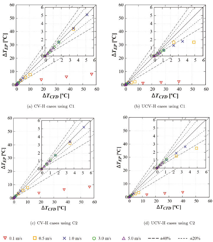
Figure 10 Comparison of ∆T from EnergyPlus and CFD simulations for H cases, and for different wind speeds and heat levels, a) and b) using C1, c) and d) using C2. Low values are enlarged in the insert. Symbols denote the wind speed at a 10 m height. For a given v10 the four heat levels can be distinguished since the values of ∆T and Q increase with the increase of the heat flux or the temperature on the floor. The dashed lines indicate the percentage error
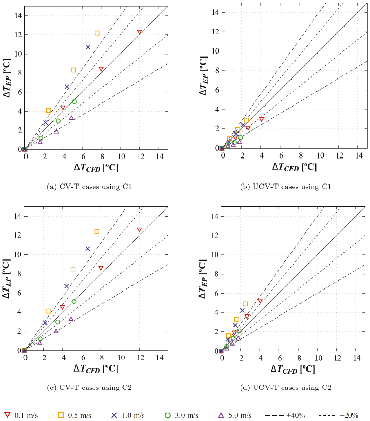
Figure 11 Comparison of ∆T from EnergyPlus and CFD simulations for T-cases, and for different wind speeds and heat levels, a) and b) using C1, c) and d) using C2. Symbols denote the wind speed at a 10 m height. For a given v10 the four heat levels can be distinguished since the values of ∆T and Q increase with the increase of the heat flux or the temperature on the floor. The dashed lines indicate the error in percentage
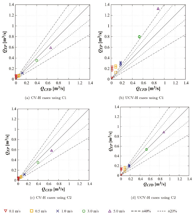
Figure 12 Comparison of Q from EnergyPlus and CFD simulations for H cases with different wind speeds and heat levels. a) and b) using C1, c) and d) using C2. Symbols denote wind speed at a 10 m height. For a given v10 the four heat levels can be distinguished since the values of ∆T and Q increase with the increase of the heat flux or the temperature on the floor. The dashed lines indicate the error in percentage
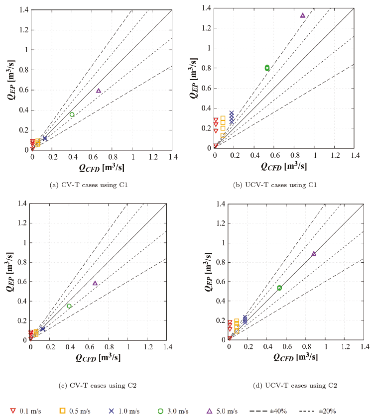
Figure 13 Comparison of Q from EnergyPlus and CFD simulations for H cases with different wind speeds and heat levels. a) and b) using C1, c) and d) using C2. Symbols denote wind speed at a 10 m height. For a given v10 the four heat levels can be distinguished since the values of ∆T and Q increase with the increase of the heat flux or the temperature on the floor. The dashed lines indicate the error in percentage
In the following paragraphs, when a pair of percentages is reported, the two results correspond to the C1 and C2 coefficient groups, respectively.
For CV-H cases (Figure 10) EP reproduces the CFD value of ∆T for v10 ≥ 1.0 m/s with a difference of less than 5 % and 4 %, for v10 = 0.5 m/s the difference is of less than 26 % and 24 %, but for v10 = 0.1 m/s the difference is of up to 86 % and 85 %.
For UCV-H cases, the difference between EP and CFD ∆T results for v10 ≥ 3.0 m/s is of less than 38 % and 8 %, for v10 = 1.0 m/s the difference is of up to 48 % and 23 %, while for v10 ≤ 0.5 m/s the difference is of up to 94 % and 91 %. For both configurations (CV and UCV) using C2 gives better results. Nevertheless, for CV-H cases the improvement is not significant. For UCV-H cases, especially for v10 ≥ 1.0 m/s, the enhancement is significant.
In H cases, EP has a better agreement with CFD for the CV configuration than it does for the UCV configuration. For both configurations the agreement increases as v10 increases.
For CV-T cases, shown in Figure 11, EP reproduces the CFD value of ∆T for v10 = 0.1 m/s with a difference of less than 9 % and 11 %, and for v10 = 3.0 m/s with a difference of less than 29 % and 28 %, for the other values of v10 the difference is up to 62 % and 64 %. For UCV-T cases, the difference between EP and CFD ∆T results for v10 = 0.1 m/s is less than 10 % and 40 %, and for v10 = 3.0 m/s is less than 45 % and 20 %. For the other values of v10 the difference is up to 64 % and 100 %. For CV-T cases the difference between C1 and C2 results is not significant, while for the UCV-T cases the difference is significant.
In T cases, EP has a similar agreement with CFD for both configurations. In both configurations the results do not show a tendency with respect to v10.
When comparing the H and T cases using ∆T, in general, the agreement between EP and CFD results is better in H cases, except for the lowest value of v10 for which T cases show a better agreement.
Figure 12 shows Q results for CV-H cases. EP reproduces the CFD value of Q for v10 ≥1.0 m/s with a difference of less than 12 % and 13 %, for v10 = 0.5 m/s the difference is less than 15 % and 13 %, but for v10 = 0.1 m/s and 750 W the difference is up to 472 % and 449 %. For UCV-H cases, the difference between EP and CFD Q results for v10 ≥ 3.0 m/s is less than 51 % and 1 %, for v10 = 1.0 m/s is up to 81 % and 22 %, for v10 = 0.5 m/s is up to 187 % and 95 %, and for v10 =0.1 m/s is up to 1,240 % and 788 %. For the CV configuration the results using C1 and C2 are similar, but for the UCV configuration the results improve significantly when C2 is used, especially for v10 ≥ 1.0 m/s. Furthermore, when using Q as the comparison variable, the agreement between EP and CFD is better for the CV configuration than it is for the UCV.
Figure 13 shows Q results for CV-T cases. EP reproduces the CFD value of Q for v10 ≥ 1.0 m/s with a difference of less than 13 % and 14 %, for v10 = 0.5 m/s the difference is up to 40 % and 35 %, for v10 = 0.1 m/s the difference is up to 601 % and 569 %. For the UCV-T cases, the difference between EP and CFD Q results for v10 ≥ 3.0 m/s is less than 52 % and 2 %, for v10 = 1.0 m/s is up to 99 % and 34 %, for v10 = 0.5 m/s is up to 234 % and 121 %, and for v10 = 0.1 m/s is up to 1,515 % and 944 %. For the CV configuration, as in the H cases, the results using C1 and C2 are similar, while for the UCV configuration, the results improve significantly when C2 is used, especially for v10 ≥ 1.0 m/s.
When using Q to compare the H and T cases, the agreement between EP and CFD results is slightly better for H cases. This improvement is more noticeable for v10 ≤ 0.5 m/s. In both types of cases (H and T), for v10 ≤0.5 m/s the difference between EP and CFD Q values increases as the heat level increases. For these values of v10, EP overestimates Q with respect to the CFD. This overestimation is larger for the UCV configuration.
In general, EP gives better results for ∆T than it does for Q, especially for the CV configuration and the H cases.
One of the reasons for the difference in results between EP and CFD could be related
to the fact that EP only predicts one or two values of
Ti for the entire thermal zone, while CFD calculates
the Ti value for each cell. To analyze this hypothesis
the spatial average of
Figure 14 shows the difference for
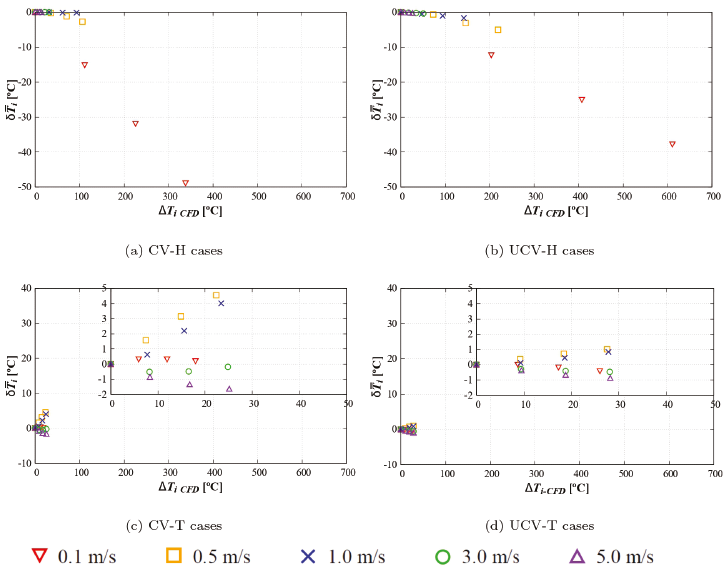
Figure 14 Difference in the average indoor temperatures from EnergyPlus (using
C1) and CFD
For T cases the values of
Figure 15 shows the percentage difference for
Q between EP using C1 and CFD simulations
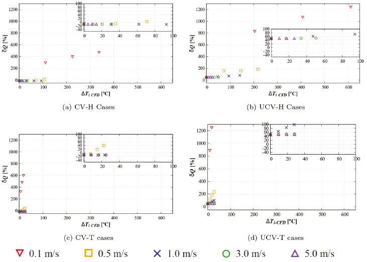
Figure 15 Percentage difference in the airflow rate Q from
EnergyPlus (using C1) and CFD (δQ) as a function of the
difference between the maximum and average indoor temperatures obtained
from CFD
Conclusions
Results of natural ventilation cases obtained from EnergyPlus (EP) simulations using the Airflow Network model (AFN) and the cross-ventilation model are compared with results from validated computational fluid dynamic (CFD) simulations. All simulations are performed in a steady state. Wind and buoyancy effects are considered for two configurations: cross ventilation (CV) and upward cross ventilation (UCV). The buoyancy effect is produced by two heating modes: fixing a constant heat flux through the floor (H) and fixing a constant floor temperature (T). For each heating mode, four heating levels are considered. Wind speed at a 10 m height (v10) is varied from 0.1 m/s to 5.0 m/s. EP results using one of two coefficient groups (C1 and C2) are compared with results from the CFD simulations. In the C1 group, the wind induced pressure coefficients Cp are calculated by EP, and the discharge coefficients Cd are taken from the literature. In the C2 group, these coefficients are obtained from the CFD simulations.
The main conclusions derived from this work are the following:
It is important to use the EP cross-ventilation model for the CV and UCV configurations. Although the temperature difference between the recirculation region and the jet region is smaller than 0.4°C, the percentage velocity difference between the jet region and the recirculation region with respect to the jet region is up to 42 %.
In the CV configuration, EP using C1 predicts good results for indoor air temperature (Ti) and airflow rate (Q) in the following conditions: v10 = 0.5 m/s and floor temperature ≤ 25°C or floor heat flux ≤ 250 W; v10 = 1.0 m/s and floor temperature ≤ 25°C or all floor heat flux levels; and v10 ≥ 3.0 m/s for all floor heat levels. EP predicts Ti with a difference of up to 1.6°C and Q with a difference of up to 12 % with respect to CFD simulations.
In the UCV configuration, EP using C1 only predicts good results for Ti in the following conditions: v10 = 0.5 m/s without heating; v10 = 1.0 m/s and all floor temperatures or floor heat flux ≤ 250 W; and v10 ≥ 3.0 m/s for all heat levels. EP predicts Ti with a difference of up to 1.0°C with respect to CFD simulations. EP overestimates Q with respect to CFD simulations. This difference is up to 52 % for all velocities without heating as well as for v10 ≥ 3.0 m/s for all heat levels.
In the CV configuration, EP using C2 coefficients gives similar results to those obtained using C1 coefficients. In contrast, the use of C2 coefficients for the UCV configuration significantly improves results, particularly for Q.
In the UCV configuration, EP using C2 coefficients predicts very good results Ti with a difference up to 0.5°C and Q with a difference up to 3 % with respect to CFD simulations) in the following conditions: all velocities without heating and v10 ≥3.0 m/s for all heat levels. EP gives satisfactory results (the differences with respect to CFD simulations are up to 2°C for Ti and up to 34 % for Q) for the cases with v10 =1.0 m/s and all heat levels.
Thus, for the UCV configuration it is recommended to use coefficients obtained from CFD simulations, instead of the Cp calculated by EP and the Cd taken from the literature.
It is recommended that the Airflow Network model be employed for practical thermal simulations of naturally ventilated buildings using EnergyPlus (EP). The cross-ventilation model must also be used for thermal zones with cross-ventilation.
The analyses made in this research show that an improvement on the natural ventilation models of EP is required, especially for low wind velocity and high heat internal gain conditions. The authors are beginning experimental and theoretical research on thermally driven natural ventilation (Castillo et al., 2021), and they expected to make a model to be incorporated in EP in the near future.
Nomenclature
Acronyms
| AFN | Airflow Network Model |
| AIVC | Air Infiltration and Ventilation Centre |
| CFD | Computational Fluid Dynamics |
| CV | Cross Ventilation |
| EP | EnergyPlus |
| NNV | Natural Night Ventilation |
| PIV | Particle Image Velocimetry |
| SPIV | Stereoscopic Particle Image Velocimetry |
| TARP | Thermal Analysis Research Program |
| UCV | Upward Cross Ventilation |
| WE | Windexchanger |
Latin symbols
| ACH | Air changes per hour [1/h] |
| Cd | Discharge coefficient [—] |
| Cp | Pressure coefficient [—] |
| K | Turbulent kinetic energy [m2/s2] |
| kS | Sand grain roughness height [m] |
| Q | Air flow rate [m3/s] |
| q | Heat flow rate [W] |
| Ti | Indoor air temperature [°C] |
| To | Outdoor air temperature [°C] |
| U | Air velocity (or water velocity) [m/s] |
|
|
Atmospheric boundary layer friction velocity [m/s] |
| Uref | Reference velocity equal to the wind velocity at the building height [m/s] |
| uref | Reference velocity equal to the wind velocity at the opening height [m/s] |
| v10 | Wind speed at a 10 m height [m/s] |
| z0 | Roughness length [m] |

