2.1 Real-Parameter Single Objective Optimization Problems

A real-parameter single objective optimization problem can be stated as follows: Given a function f(X):ℝN→ℝ, an algorithm has to find the values of the variables of a vector X such that they minimize or maximize the function f (called the objective function). In this type of problems, it is assumed that the vector X can have N variables (X=(x1, x2, …, xN)) and the search space within which the search for such a vector of variables is performed is bounded by the lower and upper bounds corresponding to each variable, i.e., ai≤xi≤bi, i∈{1, 2, …N}, where ai is the lower bound and bi is the upper bound corresponding to the variable i.

2.2 Standard Particle Swarm Optimization

The PSO algorithm was proposed by Kennedy and Eberhart in 1995 [⁴]. This optimization algorithm attempts to mimic the complex socio-cooperative behavior exhibited by different animal species such as flocks of birds and schools of fish.

The standard version of PSO [¹⁴] utilizes a swarm of NP particles, where each particle represents a potential solution to an optimization problem. This swarm is randomly placed within the N-dimensional search space of the optimization problem. For the ith particle of the swarm, its position and velocity at iteration t are denoted by Xi=(xi1, xi2, …, xiN) and Vi=(vi1, vi2, …, viN) respectively. Then the new velocity and position of this particle at iteration t+1 are calculated as follows:

where i=1, 2, …,NP, c1 and c2 are two non-negative acceleration factors, r1, r2 are two uniformly distributed random numbers, Xipbest=(p1, pi2, …, piN) is the best solution found by the ith particle itself until iteration t, and Xgbest is the best solution found by the entire swarm until iteration t. ω is the inertia weigth to balance the global and local search abilities of particles in the search space, which is given by:

where t represents the current iteration, ωmax and ωmin are the maximum and minimum limits respectively of the inertia weigth ω, and T is the maximum number of iterations. Then, the position of the particles is updated as follows:

and check that Xi,t+1 stays within the search space delimited by its boundary constraints.

In Equation (1), the first term represents the inertia of the previous velocity, the second term is known as the cognitive component and is related to the personal experience of each particle, the third term is called the social component and is related to the cooperation between particles.

2.3 Social Learning

Learning in various animal species consists of a process that allows them to acquire, store and subsequently use information from their environment. Some species, particularly those that live in groups, have developed the ability to learn from other members of their group [⁶]. Experienced individuals, such as parents, as well as long-lived and successful members, provide a reservoir of useful behaviors. Adopting behaviors from this reservoir allows new or inexperienced individuals to skip the many iterations of trial-and-error necessary for their individual learning and move directly to solutions previously tested by other individuals. Through social learning, behaviors can be transferred from one generation to the next, resulting in more complex behaviors that help to solve tasks such as foraging and predator avoidance in an efficient way [⁶, ¹⁶].

3.1 Motivation

The SL-PSO algorithm is a variant of the standard PSO algorithm that utilizes the historical information of the search process, specifically the information of the best individuals during the search process. The decision to use this information is made with the aim of mitigating the stagnation of particles within the search process, taking into account the fact that different species of animals living in groups use this information and learn from the behavior of other members of the group through social learning.

3.2 Algorithm Description

The SL-PSO algorithm incorporates an external archive called A with size NP, which stores the best part of the swarm (Xgbest,t) in each iteration. Unlike the standard PSO, which uses only information from the current generation, the proposed algorithm uses both current and historical information through A.

When the ith particle does not improve its result considering the fit value between two consecutive iterations, a stagnation counter Cs≥0 increments its value by one unit. If the stagnation counter exceeds a set threshold (δs), this particle is subjected to a social learning process in which the particle uses the historical knowledge of the best particle in the swarm to escape a possible stagnation and at the same time allows it to move towards regions with a higher improvement potential. This intervention of the social learning process implies that the position of the swarm is modified as follows:

where Xi,t is the position of the particle just when the stagnation counter Cs exceeds the set threshold, N(0, exp⁡−t/10) is a vector of the same size as Xi,t with randomly generated values from a normal distribution with zero mean and standard deviation given by exp⁡−t/10, t represents the current iteration, γ is a uniformly generated random number, and XAr,t is one of the best swarm positions randomly selected from A.

Fig. 1 shows a diagram that illustrates the proposed modification. In this diagram, a particle Xi,t (red circle) is close to a local minima, which can provoke the stagnation of the particle and thus finally activate the social learning process. In this process, the particle uses the information of one of the best particles of the swarm stored in the archive A (green circle) and a perturbation provided by the vector N(0, exp⁡−t/10). This allows the particle to modify its position (magenta circle) to a new region of the search space and to improve its orientation with respect to the best particle of the swarm within the current generation (cyan circle).

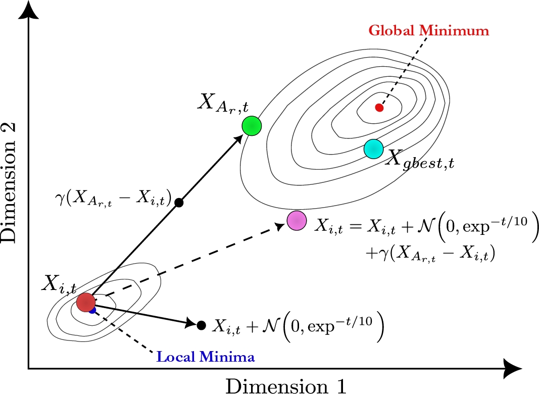
Fig. 1 Diagram showing the change in the position of a particle as a result of the process of social learning 

Once the social learning process is applied to a particle, its stagnation counter is reset to zero. It is important to note that in the Equation (4), the vector N(0, exp⁡−t/10) is intended to generate a random perturbation at the current position of the particle. Since this perturbation comes from a normal distribution with zero mean and standard deviation given by exp−t/10, the values generated for this random perturbation vector tend to values closer to zero as the evolution process progresses. Thus, at the beginning of the algorithm execution, larger perturbations are obtained, which improve the exploration capacity of the algorithm, while at later stages of the evolution process, smaller perturbations are generated, which can benefit the local search of the algorithm. It is also worth noting that the speed of the particles is not modified within the social learning process and remains equal to the value obtained just when the social learning process is activated.

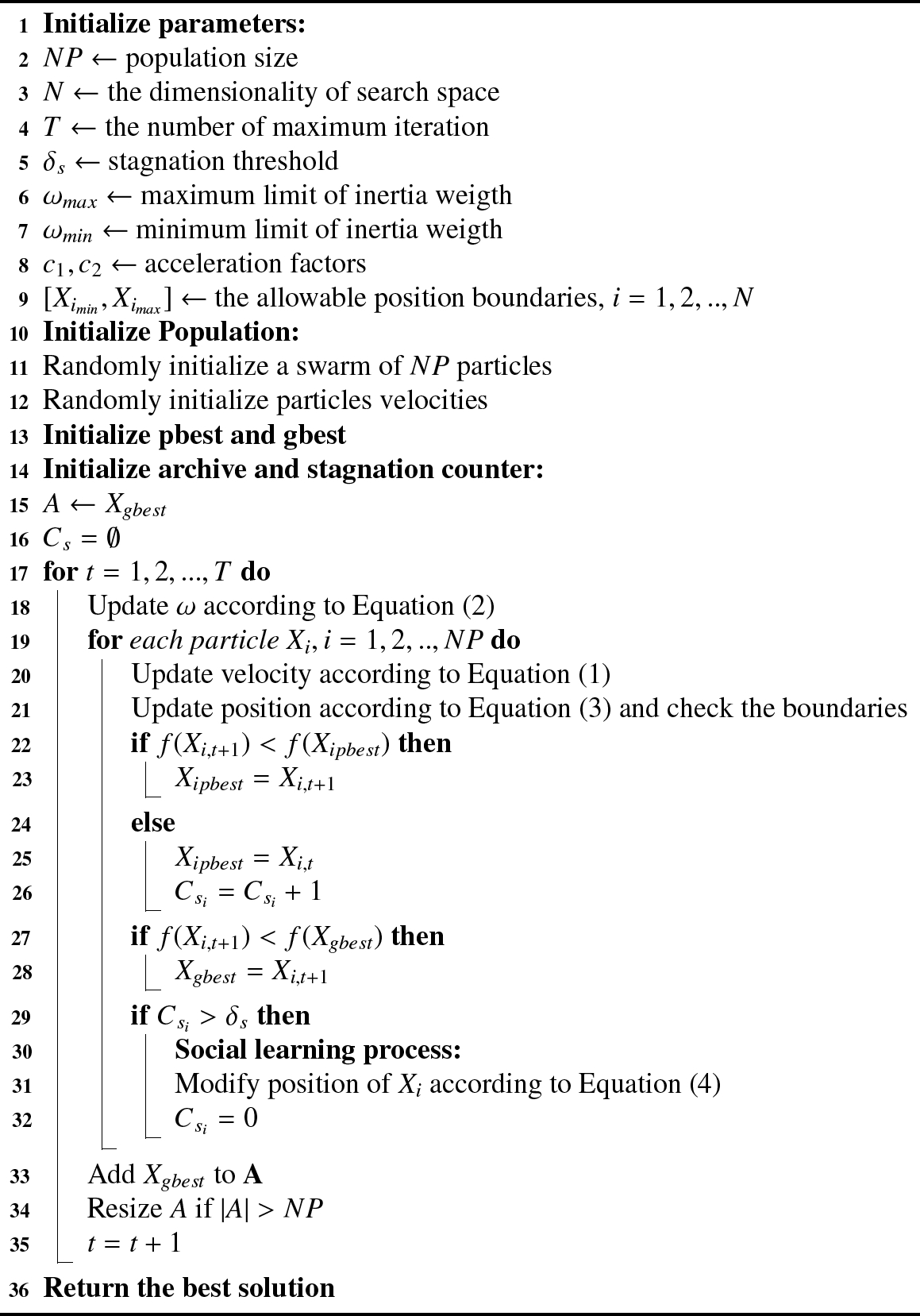
The pseudo-code in Fig. 2 provides a detailed description of the proposed SL-PSO algorithm.

Fig. 2 SL-PSO algorithm 

4.1 Benchmark Functions

To evaluate the performance of SL-PSO on different optimization problems, 10 benchmark functions were selected from the set of single-objective optimization problems with boundary constraints from the CEC2017 competition [¹⁰]. Three of the benchmark functions (F1−F3) are of the unimodal type, i.e., functions with a single global optimum, and the rest of them (F4−F10) are functions with multiple local optima, also known as multimodal functions. The corresponding dimensions, search spaces, and values of their respective global optima are shown in Table 1.

4.2 Algorithms and Parameter Settings

The experiments were conducted using Python 3.11 programming language on a computer with 8 GB of RAM and a 3.6 GHz six-core processor. The performance of SL-PSO was compared with the standard PSO, the constraint factor PSO (CPSO) [²], the human behavior-Based PSO (HPSO) [¹¹], and the PSO variant based on local stochastic search strategy (LSSPSO) [³] on the set of benchmark functions described in section 4.1.

In the simulations performed, all algorithms were run with the same number of iterations and particles: 1000 and 100, respectively. These values are commonly used in the PSO algorithm [⁹, ¹²]. For each algorithm, 51 independent runs were performed for each function with N=10 and N=30. The initial population was uniformly distributed over the search space. The inertia factor range was set to [0.4, 0.9]. Table 2 shows the configuration of the five algorithms. All the comparison algorithms adopt the authors’ suggested parameter configurations.

4.3 Comparison of SL-PSO with PSO Algorithms

Tables 3 and 4 report the statistical results of the tests performed on the five algorithms for N=10 and N=30, respectively. The solution error measure Fmin−F(X*) was used to obtain these results, where X* represents the best solution found in each algorithm repetition, and Fmin is the known solution to the problem. The mean and standard deviation of the solution error measure over 51 independent runs are shown for each function and algorithm. The best value for each function among all algorithms is shown in bold. To identify significant differences between the algorithms, the non-parametric Wilcoxon rank sum test with a confidence level of 0.05 was also implemented [¹⁵]. The values in the “W/T/L” row indicate the number of functions where the SL-PSO algorithm performed significantly better (+), similar (≈), or worse (−) than its counterpart. It is worth noting that the mean of the solutions is a measure of the solution quality of the algorithms, while the standard deviation is a measure of their stability.

According to the results presented in Table 3, SL-PSO achieves the best performance on the functions F1, F2, F3, F4, F5, F7, F8, and F10, while HPSO achieves the best performance on the functions F6 and F9. PSO, CPSO, and LSSPSO do not perform well on any of the benckmark functions. As can be seen in this table, SL-PSO ranks first among all algorithms in terms of average mean performance, while the standard PSO algorithm ranks last. SL-PSO shows significant advantages except for three functions (F6, F7, F9), but does not show significant disadvantages in any case. In addition, SL-PSO has the lowest standard deviation values for most functions, followed by HPSO.

For N=30, the results in Table 4 indicate that SL-PSO performs best on the functions F1, F2, F3, F4, F5, F8, and F10, while HPSO performs best on functions F6, F7, and F0. It is worth noting that the SL-PSO algorithm performs well on both unimodal and multimodal functions. However, none of the PSO, CPSO, and LSSPSO algorithms perform well on any of the benchmark functions. As with the results for N=10, PSO ranks last in terms of performance, with SL-PSO achieving the best performance, followed by HPSO. The HPSO algorithm presents significant advantages in functions F6, F7, and F9, while SL-PSO has significant advantages on functions F1, F2, F3, F4, and F10. In addition, SL-PSO achieves the lowest standard deviation values for the majority of functions, showing its ability to solve problems with multimodal functions.

Fig. 3 shows the convergence curves of the evolution process of SL-PSO, PSO, CPSO, HPSO, and LSSPSO. The benchmark functions F3, F6, and are used to exemplify the convergence characteristics for cases where N=10 and N=30, with T=1000 and NP=100. Each curve represents the average of 51 runs over a function, obtained by a specific algorithm.

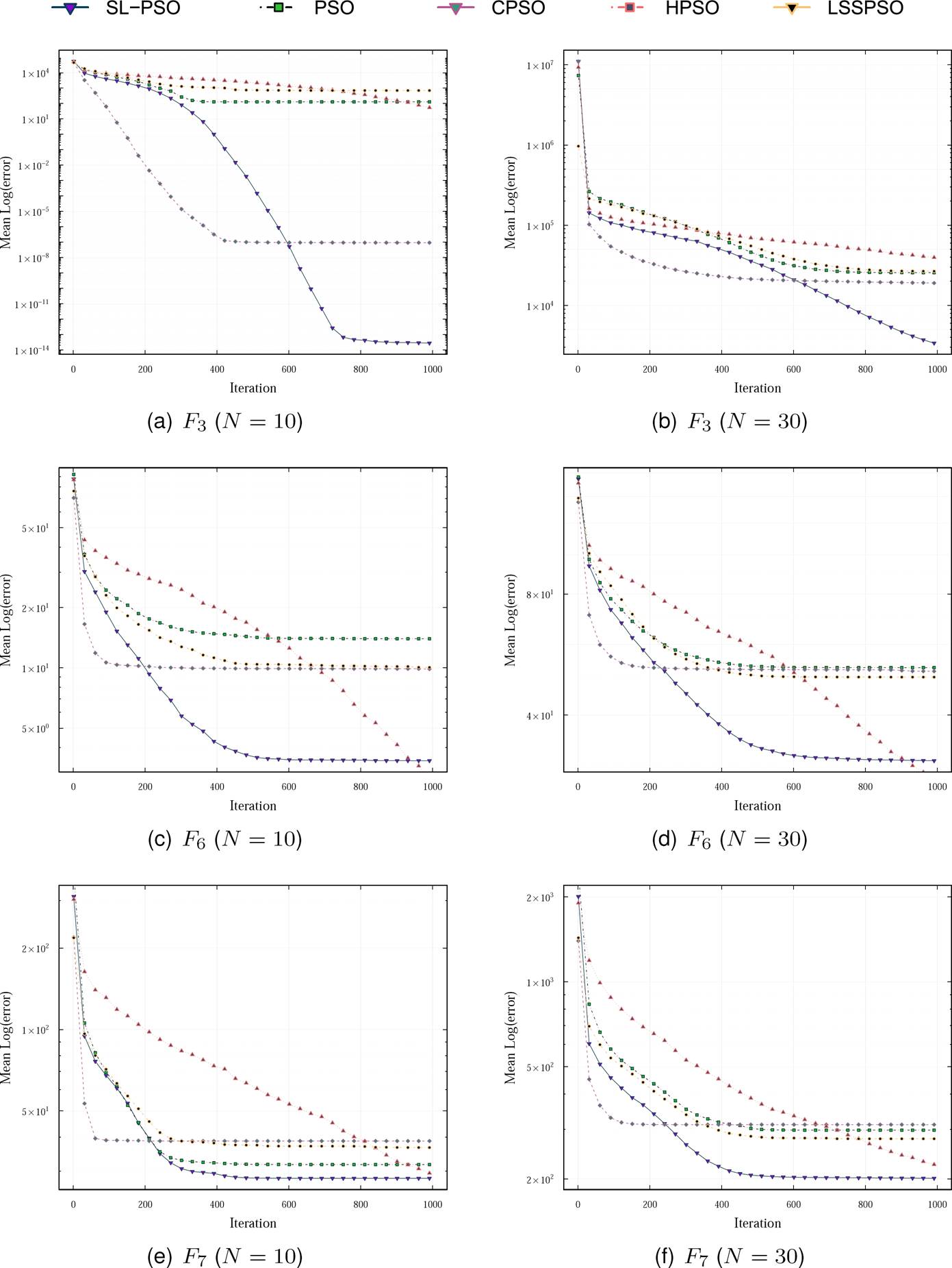
Fig. 3 Convergence curves of SL-PSO, PSO, CPSO, HPSO, and LSSPSO for the selected functions. The cases of N=10 and N=30 are considered, with T=1000 and NP=1000. A logarithmic scale has been used for visualization purposes 

Figs. 3(a) and 3(b) show that for the unimodal function F3, SL-PSO achieves the highest accuracy in both 10 and 30 dimensions, while the rest of the algorithms maintain higher average error. Figs. 3(c) and 3(d) show that for the multimodal function F6, HPSO produces the lowest mean error, while SL-PSO remains in second place. The remaining algorithms achieve higher mean errors. This behavior is observed in both 10 and 30 dimensions. Finally, Figs. 3(e) and 3(f) show that for the multimodal function F7, all algorithms keep relatively close error means in both 10 and 30 dimensions. However, SL-PSO achieves the lowest mean error, followed by HPSO.

Based on the accuracy of the solutions (Tables 3 and 4), as well as the convergence characteristics (Fig. 3), it can be clearly stated that SL-PSO significantly outperforms PSO, CPSO, and LSSPSO, in both unimodal and multimodal functions, even as the number of dimensions increases. On the other hand, SL-PSO performs competitively with respect to HPSO mainly as the number of dimensions increases.