


 nueva página del texto (beta)
 Inglés (pdf)
 Artículo en XML
 Referencias del artículo
 Enviar artículo por email
 Citado por SciELO
  Similares en
SciELO
Similares en
SciELO 
 Permalink
1 Introduction
Natural disasters are phenomena that cause significant damage worldwide. The most common ones are droughts, earthquakes, hurricanes, forest fires and floods (see Figure 1). According to the United Nations report [42], there has been a 50% increase in global floods and extreme precipitation associated with climate change. This report states that they occur four times more frequently than in the year 1980.
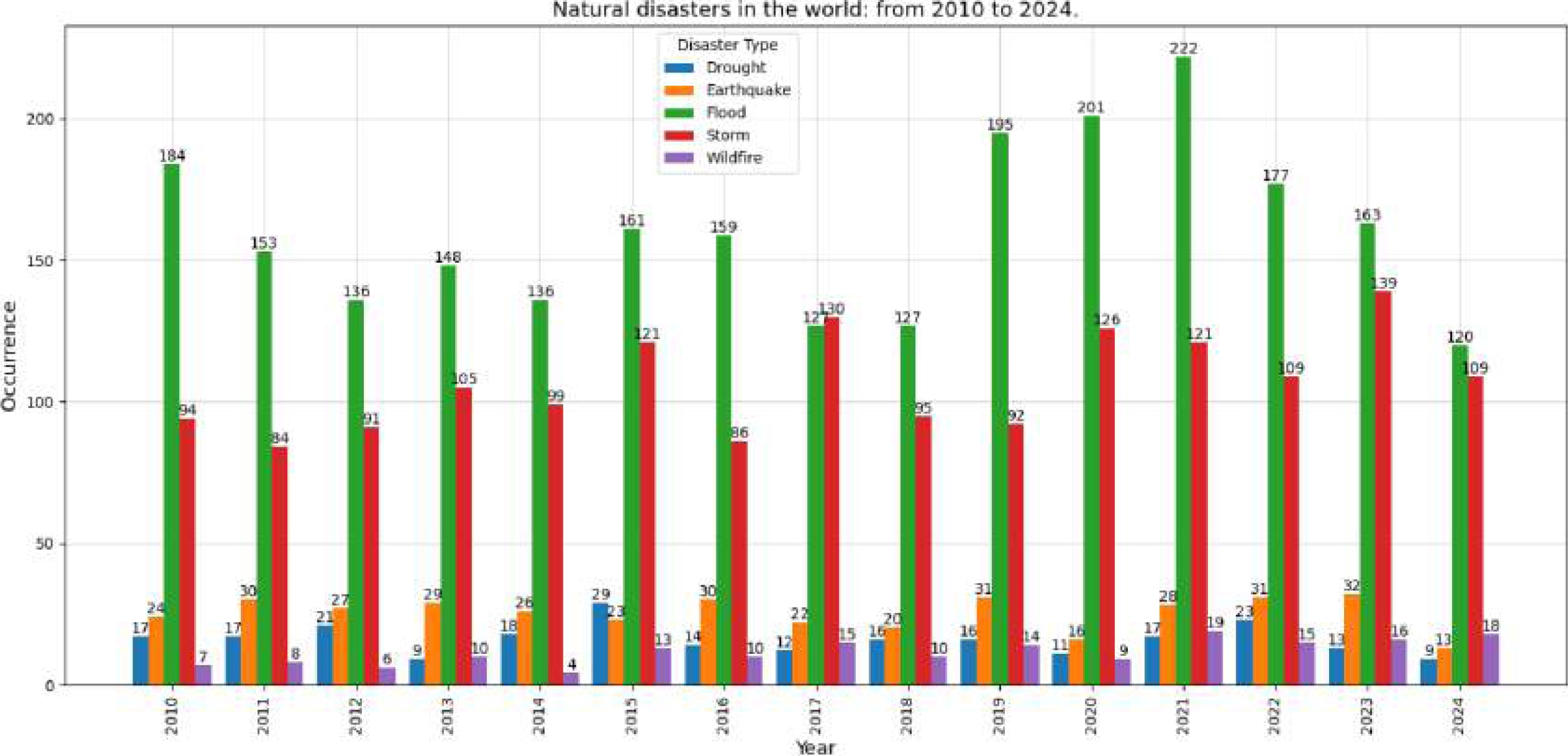
Fig. 1 Occurrence of the five most common natural disasters in the world from 2005 to 2024: Floods, Storms, Earthquakes, Droughts and Wildfires
Center for Research on the Epidemiology of Disasters (CRED) indicate that floods are the most frequent and devastating natural disaster [12]. In 2021, 432 disasters occurred, causing almost 11,000 deaths; 222 were floods (see Figure 1). In 2022, there were 387 disasters and nearly 31,000 deaths; 177 were floods. The latter have the most significant impact of these catastrophes, affecting more than 45% of the world’s population [13]. In 2023, 414 natural disasters were recorded, of which 163 were floods, leaving more than 7,500 deaths [14]. As of October 2024, 120 floods have been recorded.
In Mexico, there have been several floods that have caused severe damage. Among the most serious ones are those that occurred in the state of Tabasco in 2007 and 2020; causing a large percentage of its territorial extension to be completely covered by water. This generated impacts in different sectors, such as agriculture, livestock and infrastructure [32]. According to official data from ECLAC [10], the damage caused in 2007 was USD 3,000,000.00: 31.77% in the productive sector, 26.9% in agriculture, and 0.5% in the environment. In 2020, more than 800,000 people were affected, 200,400 homes damaged, 2000 km of land lost and more than USD 1,000,000.00 in damages.
Due to the increase and danger of floods, various research centres have taken on the task of developing different strategies to reduce the impact of these types of disasters. As a consequence, specialized techniques and technological tools are required to propose solutions that effectively respond to the crisis and mitigate the effects caused by flooding. Research in this field will not only contribute to improving preparation and mitigation capabilities, but it also lays the groundwork for a more sustainable approach to managing future flood-related disasters.
Remote sensing has seen significant growth due to its ability to obtain terrestrial data through sensors and cameras installed on satellites or satellite programs [38, 15, 28, 21]. Satellite programs typically feature two types of sensors: passive, which capture optical images, and active, focused on capturing radar images:
— Optical images are high-resolution multispectral and correlated with the open water surface. However, they can be affected by cloud presence during precipitation, making it impossible to acquire completely clean images.
— Radar images are capable of penetrating clouds and acquiring images in any weather condition. This is due to the fact that the sensors operate at longer wavelengths and are independent of solar radiation. As a result, this makes them ideal for monitoring and mapping flooding events and estimating the damage caused.
These satellite data have different properties such as: 1) Spatial resolution, which determines the area of the terrestrial surface covered by each pixel in the image; 2) Spectral resolution, which represents the electromagnetic spectrum captured by the remote sensing sensor, including the number and width of regions; 3) Temporal resolution, which determines how long satellite information can be obtained from the same location with the same satellite and radiometric resolution [26].
Among the satellite programs are Copernicus [21] and Landsat [15]. Copernicus, which stands out for the acquisition of data with high spatial and temporal resolution, is made up of 6 satellites developed for different purposes: Sentinel-1, provides Synthetic Aperture Radar (SAR) images useful for the observation of land and oceans; Sentinel-2, provides multispectral optical terrestrial images; Sentinel-3 and 6, for marine observation and Sentinel-4 and 5 for air quality monitoring [45,11,42].
On the other hand, artificial intelligence algorithms are being used in remote sensing for the analysis of satellite data. Deep learning (DL) algorithms have taken on a very important role due to their ability to discriminate data, automate and improve the accuracy of tasks such as image classification, feature detection and the generation of thematic cartographic representations [3]. They are capable of learning appropriate feature representations for spatial learning classification tasks using Convolutional Neural Networks (CNN) [3] and sequential learning using Recurrent Neural Networks (RNN) [20]. These approaches have shown better results than other techniques, however, they suffer from some problems. CNNs suffer from inductive biases while RNNs suffer from gradient disappearance [16]. In addition, satisfactory results of DL algorithms require a large dataset for training [5, 31]. Due to this need, labeled image datasets have been used.
Both technologies are being used to study climate change, precipitation, coal flow prediction, drought forecasting, detection of land use change, earthquakes, water bodies, floods, crops, etc.
2 Related Works
In the literature, there are different approaches to analyzing water bodies and floods [18, 39, 45, 29]. Many studies use optical images, SAR (Synthetic Aperture Radar) imagery, and some combine SAR with optical data. Regardless of the approach proposed, they all share a fundamental premise: analyzing floods in various locations. Some map flood extents to coordinate rescue efforts, while others analyze flood extensions to mitigate and predict their effects.
Traditional machine learning approaches typically use optical images [17, 40, 33, 25]. Among the most commonly used algorithms are: Support Vector Machines (SVM), Random Forests (RF), and Classification and Regression Trees (CART). Optical images are analyzed using spectral indices, which are based on interactions between vegetation and electromagnetic energy in the short-wave infrared (SWIR) and near-infrared (NIR) bands [2, 23]. To map water bodies and soil vegetation, primarily the Normalized Difference Vegetation Index (NDVI) [37] and the Normalized Difference Water Index (NDWI) [7] are used. Although optical sensors are highly correlated with open water surfaces, they cannot penetrate clouds, limiting their use in rainy or overcast conditions.This makes cloud-free multispectral image acquisition impossible.
Current approaches use DL, specifically CNNs. These are based on reducing dimensionality to reduce the number of parameters and preserve relative pixel locations. By increasing the depth of CNNs, their performance can improve because deep networks incorporate multi-dimensional features and classifiers in multiple end-to-end layers. Consequently, the deeper the network structure is, the richer the feature level gets.
However, the network may introduce problems such as: 1) gradient disappearance, 2) gradient explosion, and 3) network degradation. ResNet [19] was proposed, effectively mitigating network degradation and allowing more profound training of DLs through residual blocks.
Zhao et al. [47] used SAR images to classify buildings, vegetation, roads, and water bodies using TerraSAR images [6].
Other approaches, such as those of Ziyao et al. [46] and Tavus et al. [41], use the U-Net architecture [36].
Katyar et al. [22] use the Sen1Floods11 dataset with SegNet [30]. Notably, U-Net uses skip connections between different blocks of each stage to preserve the acquired feature maps. At the same time, SegNet reuses the encoder’s pooling indices for nonlinear upsampling, thus, improving the results in flood detection.
Bai [4] improved on the work using BASNet [35], an image segmentation network identical to U-Net; they combined it with a hybrid loss function (structural similarity loss), IoU loss, and focal loss.
3 Materials and Methods
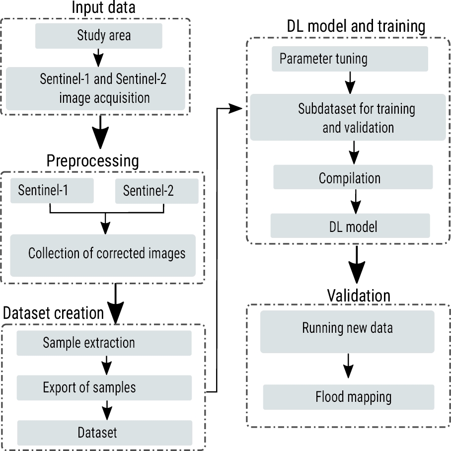
The proposed strategy has three main phases. Figure 2 shows the methodology with each of the activities of each phase. Each stage is explained below.
3.1 Study Area
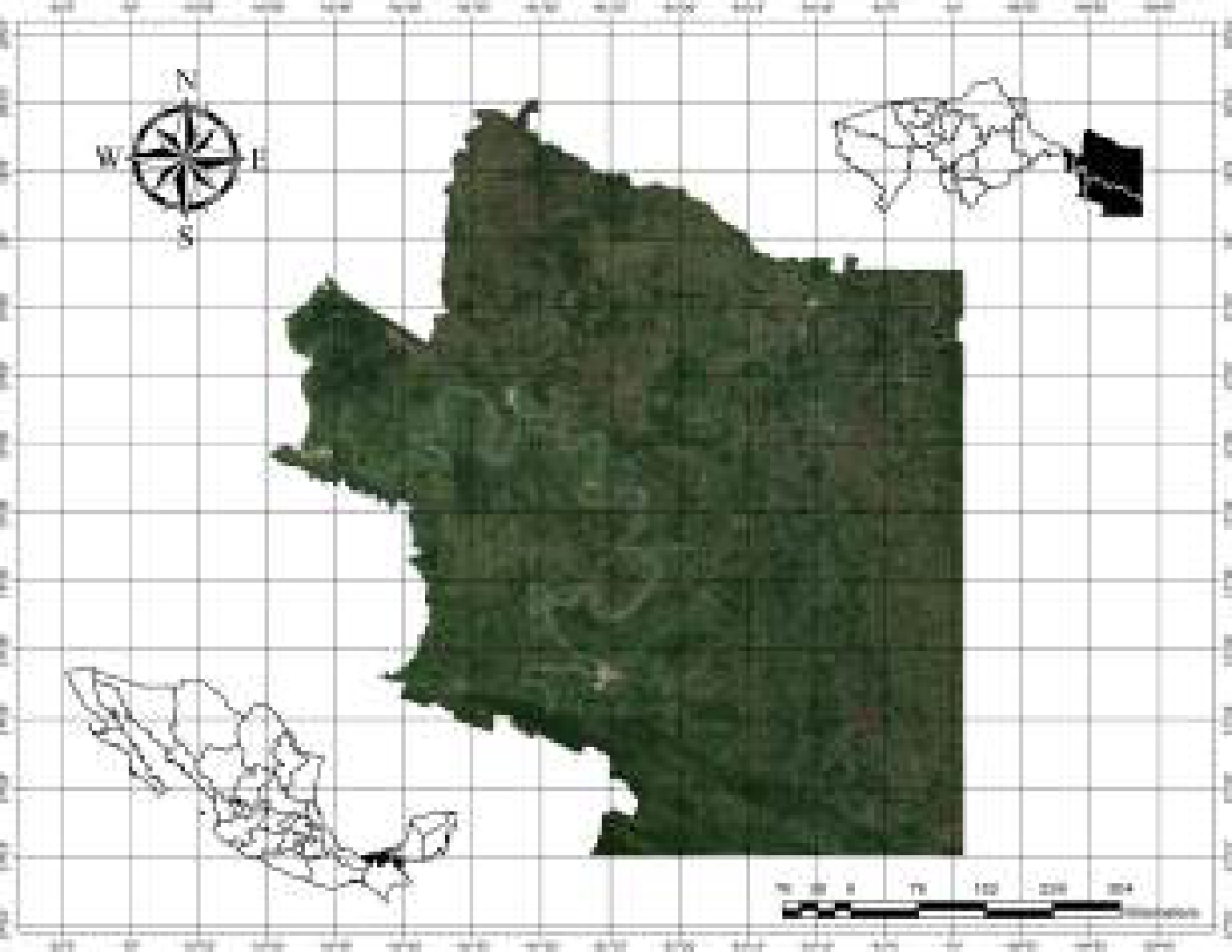
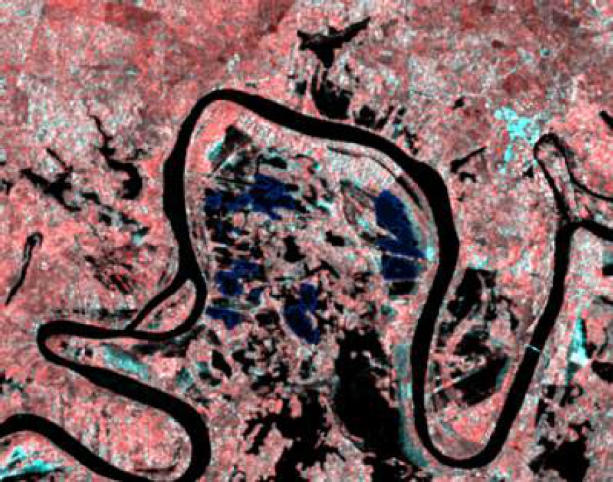
The study area focused on the river region of the state of Tabasco, Mexico. The region is composed of 3 municipalities: Tenosique, Balancán and Emiliano Zapata (see Figure 3). These entities are prone to flooding due to the large number of bodies of water that traverse the region. Additionally, it is common for prolonged rainfall to cause river overflows. The abundance of water and the impact of dams on the hydrology of the region, by altering the natural flow of rivers, cause flash floods and floods, which affect drinking water, health, and the livelihoods of thousands of Tabasco residents.
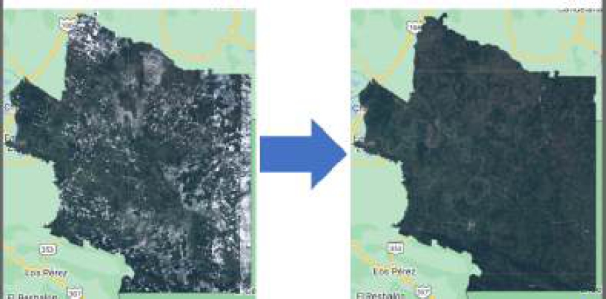
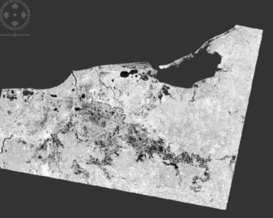
The study period was from 2020 to 2023. Three periods were established for the study: the northern season (November-February), the dry season (March-May) and the wet season (June-October). Satellite images were acquired from the Copernicus Open Access Hub repository1. Sentinel-1 images, composed of tiles covering the states of Campeche, Chiapas and Tabasco (see Figure 4), were selected; they are GRD (Ground Range Detected, focused SAR data that has been detected, multi-looked and projected to ground range using an Earth ellipsoid model) type with dual polarization VV+VH with an IW sensor.
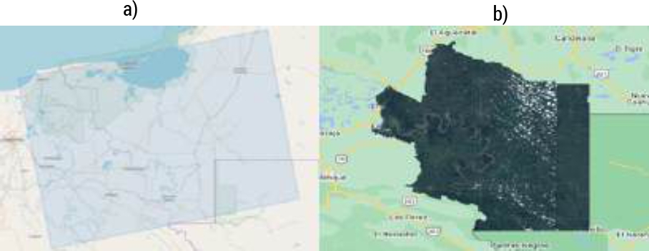
Fig. 4 Images acquired from the study area: a) Sentinel-1 image tile and b) Sentinel-2 image shapefile
Table 1 displays the parameters of the Sentinel-1 and Sentinel-2 satellite images used in the study. To avoid false positives, descending pass direction images were utilized. SAR images used for the study are shown in Figure 5. For optical images, a shapefile was used to define the study area, and the Google Earth Engine (GEE) platform was employed to acquire the images [44].
Table 1 Sentinel-1 and Sentinel-2 sensor parameters
| Satellite | Characteristics |
| Sentinel-1 | Satellite: S1-A |
| Product type: GRD | |
| Polarisation: VV + VH | |
| Sensor model: IW | |
| Sentinel-2 | Satellite: S2-A |
| Product type: 1C | |
| Cloudiness range: ¡10% | |
| Bands: 2,3,4, and 8 |
3.2 Preprocessing
3.2.1 Sentinel-1 Images
The SAR images were preprocessed using the SNAP tool and the following were applied (see Figure 7):
— Radiometric correction. Convert the information from each pixel’s original image to digital levels, and then translate these values into reflected radiance captured by the sensor. This process enables the minimization of dispersion effects caused by atmospheric particle presence [38].
— Speckle filter application. Reduce the noise characterized by speckles or small spots found in the images. A 5x5 Lee filter was employed to standardize the images and eliminate this type of noise [34].
— Geometric calibration. Correct any geometric displacement or distortion that the image presents. Distortions can be caused by sensor tilt, relief influence, or systematic errors in the image [27].
— Logarithmic scaling transformation. The image bands undergo a logarithmic scaling transformation, converting them to decibels (dB).
— RGB layer generation. An RGB mask of the SAR image was made to detect pixels where bodies of water, vegetation and flooded areas occur.
— RGB composition creation. A composition RGB (Red, Green, Blue) is generated using the image bands. Each band represents one channel of the RGB spectrum, and their combination contributes to the formation of a colored image.
— Binary layer. A binary layer is applied to segment the image, separating water and land zones by analyzing the histogram of the image’s texture coefficient. The different classes of texture coefficients are identified, and a threshold is set to separate values associated with water and land.
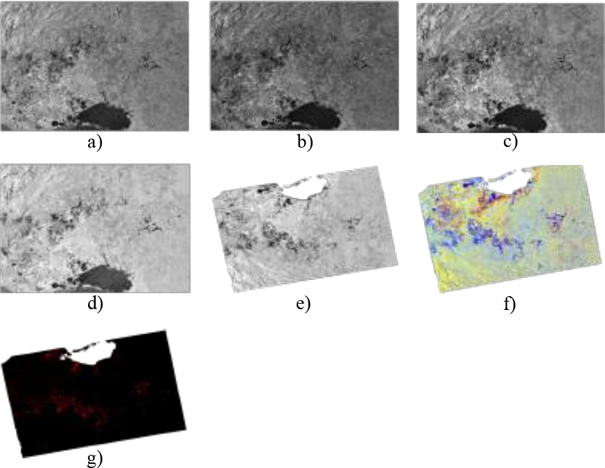
Fig. 6 SAR processing: (a) Without processing; (b) radiometric processing; (c) Speckle filtering; (d) logarithmic scaling; (e) geometric correction; (f) RGB composition; and (g) binary layer
3.2.2 Sentinel-2 Images
Sentinel-2 images at level 1C were obtained, and a cloud and shadow mask were applied to them. This mask automatically identifies and labels areas covered by clouds and shadows in the images. The mask results in cleaner images of the Earth’s surface that facilitate the study of features such as vegetation and water bodies.
Reflectance indices are dimensionless variables that result from mathematical combinations involving two or more spectral bands. The reflectance indices are designed to maximize the characteristics of vegetation and water resources but reduce noise [11, 24]. This allows analyzing the activity of vegetation and water bodies showing their seasonal and spatial changes.
Normalized Difference Water Index (NDWI). It is sensitive to changes in the content of water resources and is less susceptible to the atmospheric effects than affect NDVI, it is widely used in the analysis of water bodies [8]. It is calculated using the following formula:
where
In this stage, it is crucial to select relevant images and apply corrections to eliminate errors or deficiencies. Thanks to this, a precise and detailed understanding of the flood situation can be obtained. The final product of this phase is the collection of corrected satellite images, which provides a solid base for analysis and decision-making.
3.3 Dataset Creation
In this stage, the data is prepared for training a DL model. For this study, a CNN was employed, which is particularly well-suited for tasks related to computer vision, such as image classification and segmentation. As a result, it is necessary to create an appropriate and well-crafted dataset to provide the CNN with the necessary information to learn to identify and delineate patterns accurately and reliably, thereby achieving good performance in flood detection.
For the labeling, ArcGIS Pro [1] was used, where SAR and optical images corresponding to the established span of time for the study were utilized. The images correspond to the ríos zone in the state of Tabasco. To reduce erroneous samples, a comparison of bands from pre and post-flood images was used. All bands from both images were then stacked to generate an RGB composite. For channel
Manual samples were extracted from SAR and optical images for training purposes. This process was carried out by loading the images into ArcGIS and utilizing the ”Training Samples Manager” tool. The result can be seen in Figure 10, where polygons are drawn over a satellite image.
The training samples were exported by creating a dataset with 256×256 pixel image chips. Two separate datasets were created: one focused on flood detection and the other on permanent water bodies, utilizing SAR images and NDWI, respectively (see Table 2).
3.4 Deep Learning Model and Training
The U-Net architecture is a CNN designed for image segmentation. U-Net architecture is characterized by its efficiency in memory and computational time during inference, thanks to its smaller number of parameters. This allows the network to perform well while minimizing resource requirements. The U-shape structure enables the capture of more details and preservation of contextual information necessary for precise segmentation (see Figure 11).
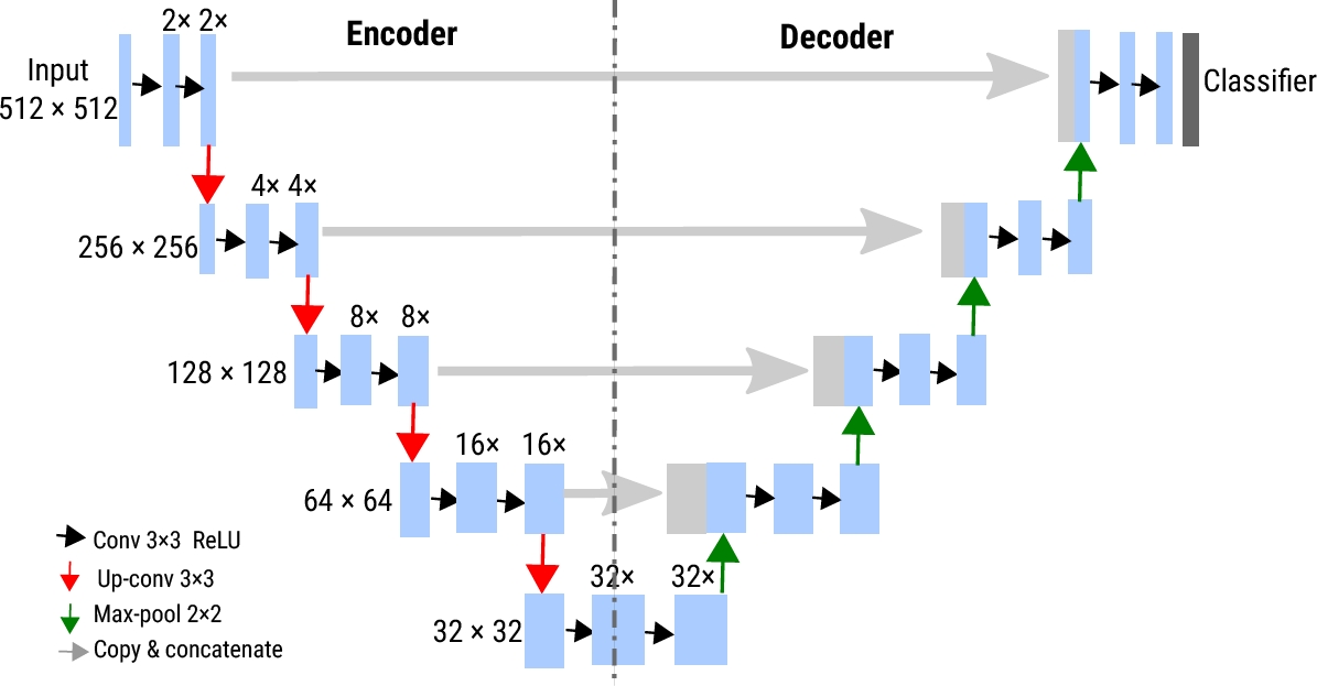
Additionally, it can handle small datasets effectively, making it particularly useful in flood mapping where dataset availability may be limited or difficult to collect. Furthermore, the U-Net architecture can benefit from techniques such as data augmentation to improve its performance. It consists of two branches: for encoding (left side) and for decoding (right side).
The encoder follows a typical CNN architecture, responsible for capturing and extracting features at higher levels of the image.
The decoder constructs the semantic segmentation map and includes convolutional layers that perform upsampling, enabling the capture of both local and contextual features.
This structure is beneficial for segmentation task, allowing the network to handle both localized and global information. The U-Net architecture uses a soft-max activation function applied in the last layer to indicate the probability of a pixel belonging to a class. It also employs a cross-entropy model to measure the discrepancy between the predicted output by the network and the expected segmentation mask or label.
The model was trained and validated using the subsets for these purposes. A batch size of 8 images per iteration was used during training. Different training tests were performed with different numbers of epochs (25, 50, 75, 100, 150, 200, 300, and 400) to evaluate performance over time. This allowed us to determine with how many epochs the best results are obtained regarding loss and precision in the validation set. Training was performed by iterating through the training batches at each iteration. Model weights are updated to minimize the loss function. Training progress is monitored, and loss and accuracy are recorded at each training and validation set epoch.
3.5 Validation
An inference test is performed to predict new flood. In this phase, the knowledge acquired during model training is applied to detect flooded areas in real-world scenarios. The key components are described below:
— Loading of the trained neural model: This step loads a pre-trained neural network model, which contains the learned weights and architecture from the training process, and is now ready to perform predictions on new images.
— Preprocess and postprocess: Preprocessing functions are used to prepare the images properly, including normalizing pixel values and adjusting the size to match the model input format. After obtaining model predictions, post-processing functions are used to improve and refine the outputs. This could involve removing small groups of unwanted pixels and improving the consistency of segmented areas.
— New image classification: Once the image has been preprocessed and the model loaded, classification proceeds. The processed image is fed into the model, generating predictions on areas that may be flooded. The model leverages its prior understanding of patterns learned during training to make these predictions.
— Visualization of results: The model’s predictions can be visualized by overlaying them on the original image. This allows for a visual evaluation of how the model has identified flooded areas in comparison to reality. The overlay also provides an indication of the quality of segmentation and potential areas for improvement.
4 Obtained Results
The following metrics were selected to evaluate the developed neural model: Recall, F1-Score, and Accuracy [43].
— Recall: Measures the proportion of positive instances (flooded areas) that the model correctly identified compared to the total number of real positive instances. A high recall indicates the model’s ability to detect most of the flooded areas in the SAR image.
— F1-Score. Metric that combines the precision and recall of the model. It measures the ratio between true and false positive predictions compared to the actual labels. It is advantageous when there is an imbalance between classes, such as in segmenting flooded areas where non-flooded areas are predominant.
— Accuracy. Evaluates the overall accuracy of a classifier. Indicates the overall performance of the model.
These metrics were evaluated in different training epochs. The model’s improvement can be observed throughout each epoch and the equilibrium points where performance stabilizes. In addition, it allows for identifying the stage where the model achieves an optimal balance between precision and recall.
4.1 Results in the Detection of Permanent Water
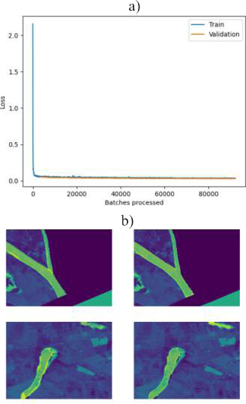
NDWI facilitated the precise identification and labeling of permanent water regions. With a training cycle of 30 epochs and 10% validation, an excellent level of evaluation metrics was achieved: precision of 91.11%, recall of 90.32% and F1-Score of 90.71%.
Figure 12.a shows the loss during training and validation. The loss represents the model’s adjustment to its predictions against real data. A low loss in both phases indicates effective learning. Figure 12.b displays samples of the trained model, with the truth of the terrain on the left and the model’s predictions on the right. Close alignment between predicted areas and sample inputs indicates precise and robust detection.
4.2 Results in Detecting Flooded Areas
For flood detection, SAR images were employed due to their ability to penetrate atmospheric conditions and provide surface terrain data, even in darkness or cloudiness. These images are ideal for this task because they can penetrate weather conditions and provide precise data on the surface terrain, even in dark or cloudy conditions. To train the model, a progressive process was used, with iterations of 25, 50, 75, 100, 150, 200, 300, and 400 epochs, at a validation rate of 10%. This progressive approach enabled the model to learn more effectively and improve its predictions in flooded areas. In Figure 13, the model’s predictions for flooded areas are displayed.
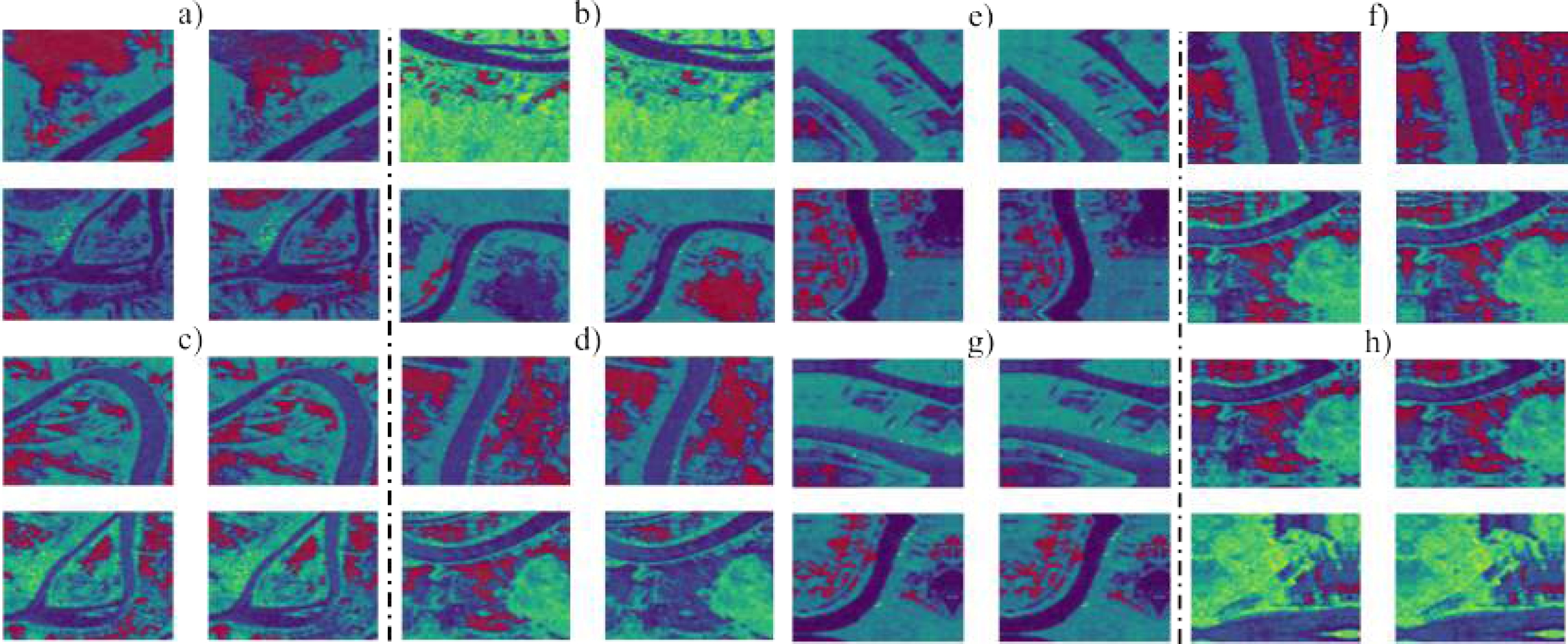
Fig. 13 Comparison of flooded areas: a) 25 epochs, b) 50 epochs, c) 75 epochs, d) 100 epochs, e) 150 epochs, f) 200 epochs, g) 300 epochs, and h) 400 epochs. Ground truth samples (left) and model prediction (right)
From epoch 150 onwards, a strategy was implemented to increase the available dataset size by implementing the rotation technique. The rotation technique was chosen because it allows for generating new samples that are not present in the original dataset, which can help improve the model’s accuracy. The new versions of each natural image were generated by applying 90-degree rotations at specific intervals, resulting in three different versions per original image. This strategy significantly enriched the training dataset (increasing from 1215 to 4860 images), introducing a greater variety and number of samples. By doing so, the model was able to learn more effectively and improve its precision in detecting flooded areas.
During the training process, it was observed that there was a gradual improvement in the model’s accuracy as the number of epochs increased. This suggests that the model effectively adapted to the greater volume of data and refined its parameters, leading to improved performance.
4.3 Classification Accuracy
During the evaluation of our model, we observed variations in the values of evaluation metrics. These variations can be attributed to several factors, including the complexity and diversity of the training data, the suitability of the model architecture or hyperparameter configuration. Despite these variations, we achieved favorable results for flood detection, particularly with increased amounts of data and extended training epochs. Table 3 presents the following evaluation metric results for each trained model.
Table 3 Comparison of the model DL’s evaluation metrics by epoch number
| Class: Permanent water | ||||||||
| Epochs | ||||||||
| 30 | ||||||||
| Accuracy | 91.11% | |||||||
| Recall | 90.32% | |||||||
| F1-Score | 90.71% | |||||||
| Class: Floods | ||||||||
| Epochs | ||||||||
| 25 | 50 | 75 | 100 | 150 | 200 | 300 | 400 | |
| Accuracy | 54.76% | 68.28% | 71.63% | 70.74% | 80.49% | 85.52% | 92.12% | 92.14% |
| Recall | 35.83% | 56.58% | 72.06% | 49.39% | 77.07% | 76.50% | 88.42% | 86.78% |
| F1-Score | 43.32% | 61.88% | 71.85% | 58.17% | 78.74% | 80.76% | 90.23% | 89.38% |
4.4 Map Generation
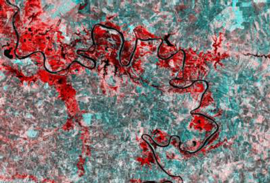
Flood Maps were created for the years 2019-2023. These maps concentrate on the northern season, spanning September, October, and November each year. Figure 14 displays some generated maps with water body extensions. The blue pixels represent permanent bodies of water, while the red pixels indicate temporary waters associated with flooding events. Table 4 reveals the territorial extent of inundated areas.
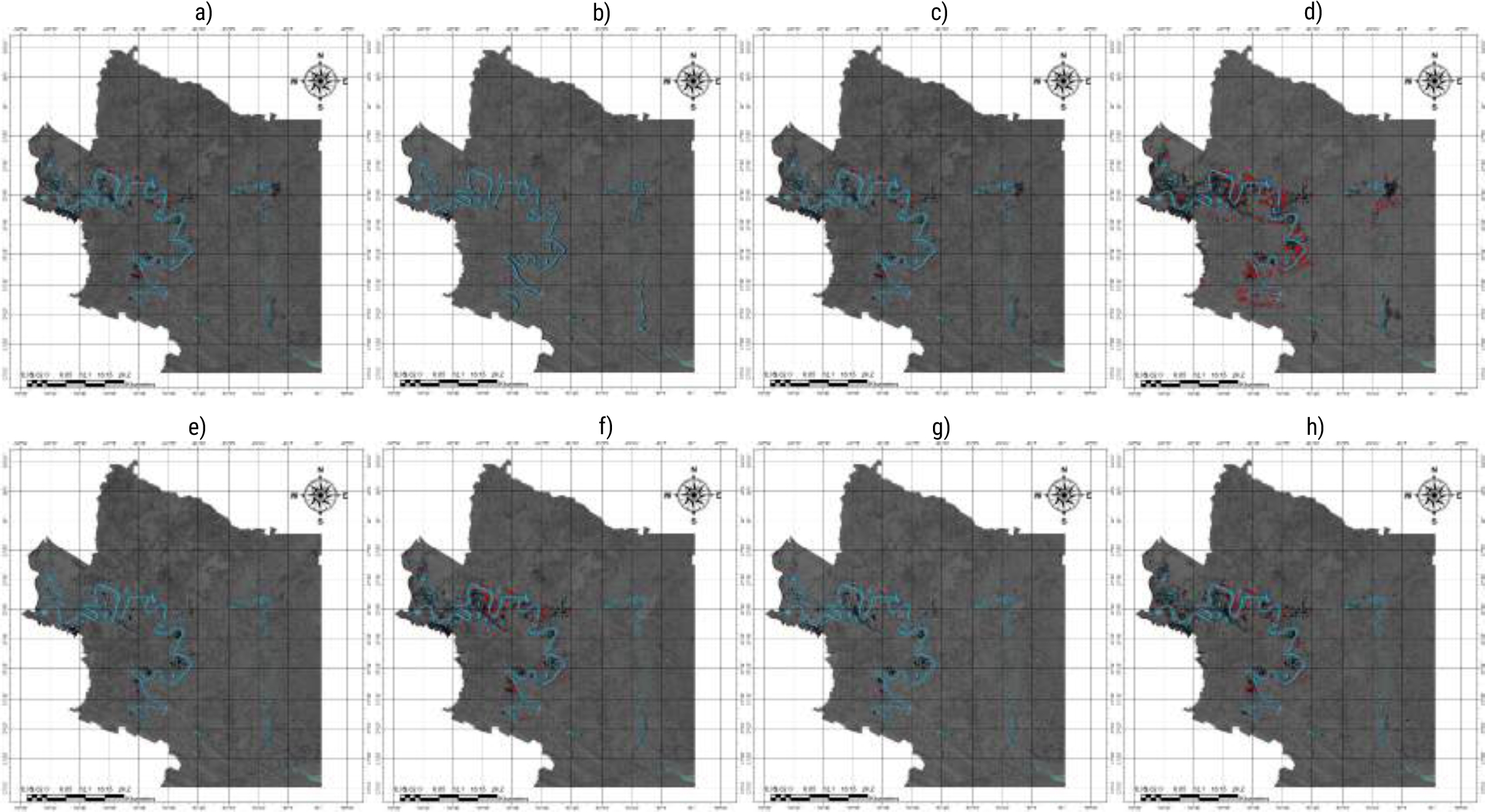
Fig. 14 Flood maps: a) September 2019, b) October 2019, c) September 2020, d) October 2020, e) September 2021, f) September 2022, g) October 2022 and h) November 2023
Table 4 Territorial extension of floods (hectares): 2019-2023
| Mes | 2019 | 2020 | 2021 | 2022 | 2023 |
| Sep | 60.93 | 1,223.62 | 120.94 | 2,680.17 | 115.94 |
| Oct | 84.77 | 475.12 | 313.58 | 2,946.25 | 120.47 |
| Nov | 78.41 | 8,175.09 | 66.93 | 371.07 | 2,576.57 |
4.5 Model Comparison with Government Flood Data
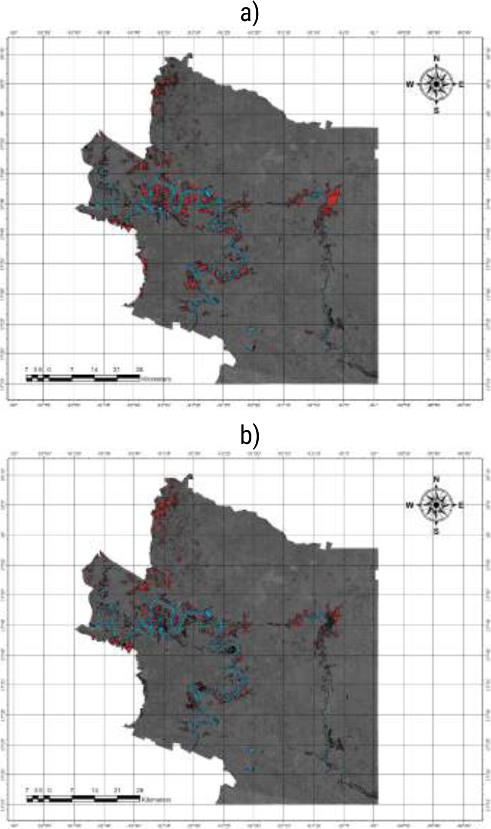
To compare the model’s performance with government data, maps of flood inundations provided by the National Center for Disaster Prevention (CENAPRED) [9] were considered. The June 2020 flood caused by Tropical Storm Cristóbal was also considered in the validation process. The comparison was carried out by visualizing CENAPRED and model maps, and quantifying flooded areas in each case. By comparing the extent and location of the areas detected by the model with those registered by CENAPRED, the accuracy and reliability of the model were verified.
CENAPRED detected 21,196.15 hectares (Ha) of flooded areas, while our model estimated 15,002.72 Ha. This results in a margin of error of 29.22% for the model, indicating that our estimation was approximately 29.22% outside of CENAPRED’s reported value.
5 Conclusions
The results demonstrate the significance of satellite missions like Copernicus, which provides free satellite data for use in various applications, including environmental monitoring and disaster prevention. The satellite images used in this study present some differences: SAR images can be obtained regardless of weather conditions, unaffected by events such as rain, clouds, etc.
Optical images are sensitive to cloud cover and require specialized techniques to obtain clear images. Combining satellite images with deep learning algorithms yields favorable results in flood detection. The combination of these technologies and tools enabled the identification of flooded zones in new datasets. It is worth noting that the lack of suitable hardware slows down model training. To improve the model, it requires being trained with a larger dataset and more epochs.

