


 nueva página del texto (beta)
 Inglés (pdf)
 Artículo en XML
 Referencias del artículo
 Enviar artículo por email
 Citado por SciELO
  Similares en
SciELO
Similares en
SciELO 
 Permalink
1 Introduction
Over the years, dealing with complex problems has motivated researchers to design and implement more powerful problem-solving techniques. However, the increase in the capacity to deal with challenging problems has paid a price: an increase in the computational resources needed to develop such strategies. In this regard, reusing solvers that require low resource consumption seems a good idea, assuming it is possible to get the best out of such solvers while benefiting from their simplicity.
In this context, the current challenges have developed a suitable playground for developing and testing algorithm selectors. Algorithm selectors are high-level strategies that manage sets of algorithms (usually simple yet valuable strategies such as heuristics), allowing them to run interchangeably, avoiding the single selection of a poor individual algorithm [19, 31].
The current literature contains various examples of implementations inspired by the algorithm selection rationale. Although using different names, it is worth highlighting: algorithm portfolios [3, 9, 19, 25], hyper-heuristics [15, 17, 26], and adaptive algorithms or adaptive algorithm selection [16, 29]. Without any loss of generality, this work will refer to any of these techniques simply as algorithm selectors.
The demand for algorithm selectors that optimize how existing straightforward techniques are used has increased. Among the many ways such algorithm selectors can be implemented, there is an observable trend in the literature to power such algorithms with machine learning models [22, 28, 35]. When algorithm selectors are implemented using machine learning (ML) models, the process can be treated as a supervised learning scenario, in which the algorithms are provided with a set of labeled examples to train the models. Once these models are trained, they can be used to solve unseen cases to estimate their performance. As described, it is possible to model the algorithm selection problem as a classification scenario that requires learning the problem features (classifier’s input) that map to a suitable algorithm to apply (classifier’s output).
Although many combinatorial optimization problems are suitable to test the approach described in this document, a very popular and straightforward one was chosen: the One-Dimensional Bin Packing Problem (BPP) [8, 12, 20]. In its simplest formulation, the BPP manages an infinite number of containers with the same capacity and a finite set of items, each with a specific weight. Solving the BPP requires packing all the items using the fewest containers possible without exceeding their capacity. This work implements algorithm selectors as classifiers that learn to map the problem features to a suitable heuristic for the BPP. The algorithm selectors receive a set of instances; for each instance, they can access the features that characterize such an instance. Additionally, for each instance, the algorithm selectors can access the individual results of each heuristic on that particular instance. At this point, it should be clear that the algorithm selectors can identify the best-performing heuristic per instance (since they know the results of each heuristic for every instance), creating a training case that maps the problem features to the label corresponding to the best heuristic for those problem features.
Commonly, datasets used for machine learning tasks contain missing values [30]. However, it seems unlikely to observe such values when the results are computer-generated through simulation, as is the case with this test problem. Although unlikely to occur, it is clear that missing one or more of the individual results from the heuristics may bias the selection of the best-performing heuristic per instance. In this context, missing values do not represent a problem but an opportunity to reduce the computational resources needed to generate algorithm selectors. Thus, missing values are introduced on purpose. The rationale behind having missing values on the individual results of the heuristics is that they may represent a way of saving computational resources. In other words, if the idea is to create a training table for
This work builds upon a previous research that explored the impact of missing values when using machine learning models as algorithm selectors [23]. In this study, we expand the scope of the previous research by including various machine learning models as algorithm selectors. To test our hypotheses, we use the one-dimensional Bin Packing Problem (BPP).
We summarize the rest of this document as follows. Section 2 provides an overview of this study with respect to related works. In Section 3, we describe the solution model. We describe the experiments conducted and analyze their main results in Section 4. Finally, Section 5 presents the conclusion and provides potential paths for future work.
2 Related Work
The literature is rich in options for implementing algorithm selectors. We can find relatively recent examples of these selectors powered by evolutionary computation [4, 18], reinforcement learning [37, 40], Simulated Annealing [32, 34], and fuzzy logic [21], to mention a few. However, we are particularly interested in implementing algorithm selectors that work as classifiers —they receive an instance characterization and return a suitable algorithm to apply.
Although we lack space for an exhaustive review of the literature on ML-based algorithm selectors, specifically those that work as classifiers as previously described, the following lines provide a chronological overview of some of the most significant works related to this topic.
Guo and Hsu studied how machine learning could be applied in algorithm selectors for NP-hard optimization problems (where NP stands for non-deterministic polynomial). They tested their approach on the Most Probable Explanation Problem in probabilistic inference [10]. Li et al. combined neural networks and logistic regres-sion to produce problem-independent algorithm selectors [14]. A few years later, Ortiz et al. explored using Learning Vector Quantization (LVQ) Neural Networks to choose which heuristic to use when solving constraint satisfaction problems [24]. Tyasnurita et al. produced algorithm selectors for the Open Vehicle Routing Problem. They used a Time Delay Neural Network to extract the patterns within the training data so the algorithm selector could work as a classifier on unseen instances [39]. Ortiz et al. proposed a framework for generating and evaluating algorithm selectors for Constraint Satisfaction Problems using various machine learning models [22]. Tornede et al. investigated meta-learning approaches to aid algorithm selection for the Boolean Satisfiability Problem [38]. Among the more recent studies, Mohamad et al. examined the use of recurrent neural networks to address the sequential aspects of combinatorial problems such as the Bin Packing Problem [1]. Additionally, Diaz et al. utilized attention-based neural networks as meta-learners to improve the performance of the mapping mechanism in algorithm selection [7]. We end this brief review with Salama et al., who proposed a Support Vector Machine (SVM) classifier with a radial basis function kernel to select the most promising dispatching rule within the Job Shop Scheduling problem, claiming to obtain savings in the computational budget concerning similar selectors implemented via Genetic Programming [33].
3 Solution Approach
The solution approach proposed produces algo-rithm selectors using various popular machine learning models: Repeated Incremental Pruning to Produce Error Reduction (RIPPER), Decision Tree (DT), k-Nearest neighbors (kNN), Support Vector Machines (SVM), Naïve Bayes Classifier (NB), and Neural Networks (NN). Once we train such models, they are ready to solve a BPP instance. They read the problem state (considering the problem features) and recommend a suitable heuristic to use given the current problem state.
The solution approach requires to generate and preprocess the data before we can apply the machine learning strategies. The following lines describe these steps.
3.1 Instance Generation
The repository contains 2000 BPP instances gen-erated using an evolutionary approach proposed by Plata et al. [27]. These instances exhibit the peculiarity of being suitable for particular heuristics and harmful to others. So, the repository contains instances that are best solved using only one of the heuristics, allowing for a balanced set where each heuristic is the best option for only a fraction of the data set. We use four techniques in this work. Then, 25% of the training set is best solved by each heuristic.
We have divided the instances into two exclusive sets, each containing 1000 instances. All the instances in these sets contain 100 items, a bin capacity of 128 units, and a maximum item length of 64. The first set was used for training purposes (undergoing various preprocessing steps that will later be described), and the second test was used exclusively for testing purposes. These instances are publicly available here1.
3.2 Heuristics
We solved each instance in the repository using four commonly used heuristics [23]. In all cases, the heuristics work with only one item at a time, and their task is to select the bin where the current item is to be packed. A short description of the heuristics used in this work is as follows:
First Fit (FF) looks for the first available bin with enough capacity for packing the item.
Best Fit (BF) looks for a bin that minimizes the waste when packed.
Worst Fit (WF) prefers the bin that maximizes the waste when the item is packed.
Almost Worst Fit (AWF) packs the item in the bin with the second most waste produced.
If there is no bin where we can pack the current item, the system opens a new bin for it. In the event of ties, the first bin that meets the heuristic’s criteria is preferred.
3.3 Problem Characterization
The one-dimensional Bin Packing Problem (BPP) is straightforward to formulate, but this simplicity comes with limitations. For instance, the only feature available for the items is their length. Therefore, to characterize the instances, we rely on basic features related to the lengths of the items. In this work, we have used five of such features. LENGTH measures the average length of the items within the instance (this value is normalized by dividing the actual average by the maximum length of items considered for this work, 64).
STD measures the standard deviation of the length of the items (also divided by 64, the maximum length allowed for the items). VSMALL represents the proportion of “very small” items in the instance (items with a length smaller or equal to 15% of an empty bin’s capacity).
Similarly, SMALL represents the proportion of ‘small’ items in the instance (items with a length larger than 15%, but smaller than 35% of an empty bin’s capacity), and MEDIUM represents the proportion of ‘medium’ items in the instance (items with a length larger or equal to 35% of an empty bin’s capacity). These thresholds were chosen based on preliminary observations. It is worth noting that the maximum item length is 64, which is half the capacity of an empty bin. Therefore, there is no need to account for ‘large’ or “very large” items.
3.4 Data Preparation
The rationale behind this work is to validate if machine-based algorithm selectors can be produced without a significant performance decrease when some individual heuristics results are missing. If this is the case, we could save resources by omitting a few results (saving some calculations).
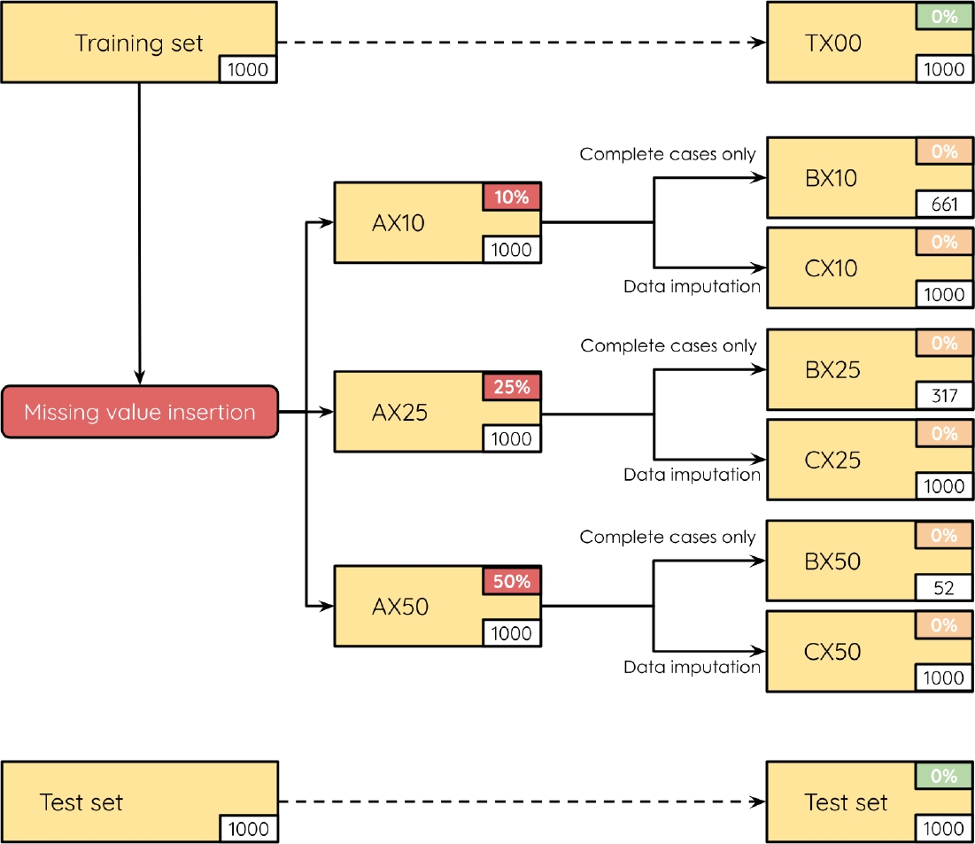
The first split of 1000 instances produced will be referred to as TX00. This set contains all the available training data (no missing values). The second split, the one devoted to testing the algorithms, will be referred simply as the test set.
Taking TX00 as a basis, we gradually introduced missing values into the results obtained by the heuristics on TX00. This way, we produced three training sets based on the proportion of missing values introduced: AX10 (10%), AX25 (25%), and AX50 (50%).
Since we intentionally eliminate some individual results from the heuristics to generate the missing values, the probability that a result is missing is the same for all the heuristics. According to the theory related to missing values, we deal with the most straightforward case, when values are Missing Completely at Random (MCAR) [11].
It is relevant to remind the reader that introducing missing values affects only the values of the heuristics and does not affect the 1000 instances from the test set. Then, the values related to the features that characterize the instances and the test set remain unaffected and complete.
After creating the three training sets with varying proportions of missing values (AX10, AX25, and AX50), we generated two new versions of each set: one where only complete cases were retained (by removing any rows with missing values), and another where missing values were imputed using the median bin usage per heuristic.
These approaches represent two fundamental techniques for handling missing data. Finally, for each version of the sets, we identified the best heuristic based on the available results for each instance. At this point, the data is ready to train the classifiers. A graphical depiction of the instances considered for this work is shown in Figure 1.
3.5 The Classifiers
he solution approach described in this document employs various classifiers. Each classifier possesses distinct characteristics and applications, allowing for a versatile and robust predictive modeling framework.
A brief description of these classifiers is provided in the following lines:
— RIPPER is a rule-based learner that generates a set of production rules from the training data [6]. It is known for its speed and efficiency, especially in managing large datasets. Ripper is particularly advantageous in contexts that require interpretable mod-els, as experts can easily understand the generated rules. This work uses the ripper implementation,
—
— Decision trees (DT) construct a tree-like structure resembling a flowchart to represent decisions based on feature values [5]. This intuitive model offers clear interpretability, making it suitable for exploratory data analysis. To implement the decision trees in this work, the function
— Support Vector Machines (SVM) are robust classifiers that function by finding a hyperplane that effectively separates different classes in the feature space [2]. For this work, the implementation of the SVMs use the most common kernels: Support Vector Machine with a Linear kernel (SVM-L), Support Vector Machine with a Polynomial kernel (SVM-P), and Support Vector Machine with a Gaussian kernel (SVM-G). To implement these three SVMs, we used the function
— Naïve Bayes (NB) is a probabilistic classifier based on Bayes’ theorem and assumes independence between features given the class label [41]. The NB classifier was implemented using the function
— Neural networks (NN) are inspired by the human brain [13]. They excel in capturing complex patterns and relationships within data, making them suitable for various applications, particularly in image and speech recognition. We implemented the neural networks as multi-layer perceptrons using the function
Each of these classifiers brings unique strengths to the solution approach, and their performance will be assessed through the accuracy obtained on the various datasets considered for this study.
4 Experiments and Results
The experimental setup consists of four experiments, described below. All the experiments were implemented using the R programming language (version 4.1.2 – “Bird Hippie”) and ran on a 4-core Linux Mint computer with 16 GB of RAM.
4.1 Training with all the Data Available
In this experiment, the idea was to produce eight algorithm selectors using the set TX00, which contains 1000 BPP instances and no missing values. The results will be used as a reference when training with missing values. To determine the best heuristic, the process chooses the heuristic with the largest bin usage for each instance.
As shown in Figure 2, all the classifiers outperform the individual heuristics. Actually, by looking at the notches from the boxplots, there is statistical evidence that supports, with 95% of confidence, that each of the classifiers is better (in terms of bin usage) than the four heuristics (on an individual pairwise comparison).
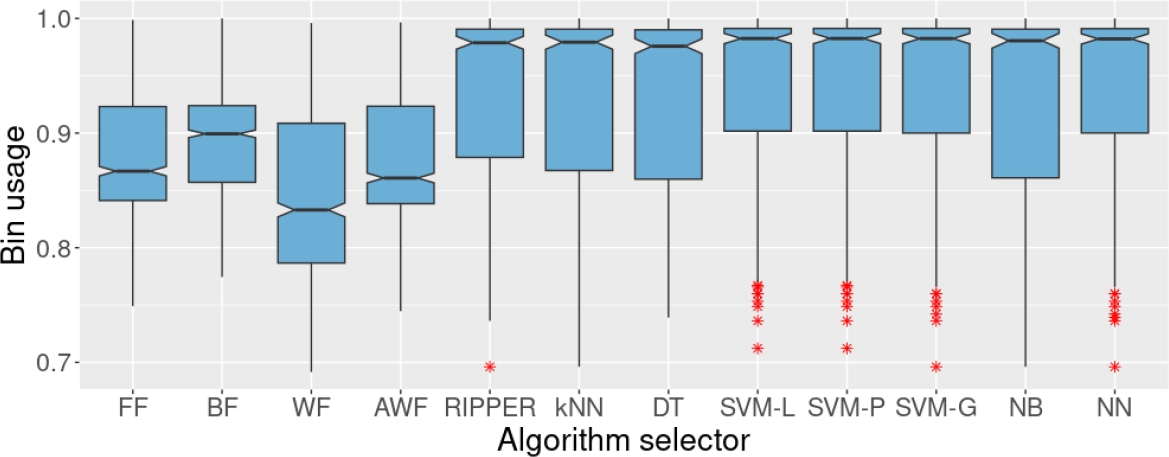
Fig. 2 Bin usage of the four heuristics and the algorithm selectors on the test set. These algorithm selectors were trained on set TX00 (that contains no missing values).
Among the algorithm selectors produced, SVM-L and SVM-P obtained the best accuracy, with 66.5% of correctly classified cases. The accuracy obtained by the remaining methods in this experiment is shown in Table 1.
Table 1 Accuracy obtained by each of the methods under study on the various test sets in this work. The best result per classifier is highlighted in bold.
| TX00 | AX10 | AX25 | AX50 | BX10 | BX25 | BX50 | CX10 | CX25 | CX50 | |
| RIPPER | 59.8% | 53.5% | 41.5% | 27.4% | 53.2% | 53.1% | 36.3% | 53.4% | 46.8% | 32.2% |
| kNN | 57.4% | 56.0% | 50.3% | 43.2% | 58.5% | 56.4% | 51.2% | 57.6% | 53.3% | 42.2% |
| DT | 60.0% | 59.2% | 58.6% | 55.6% | 59.2% | 59.0% | 49.7% | 59.7% | 59.3% | 25.0% |
| SVM-L | 66.5% | 66.2% | 66.4% | 55.3% | 66.6% | 65.2% | 59.0% | 66.4% | 62.0% | 25.0% |
| SVM-P | 66.5% | 66.2% | 66.4% | 55.3% | 66.6% | 65.2% | 59.0% | 66.4% | 62.0% | 25.0% |
| SVM-G | 66.2% | 66.6% | 65.9% | 57.9% | 65.4% | 63.5% | 56.2% | 66.8% | 64.6% | 32.8% |
| NB | 61.3% | 60.4% | 59.3% | 58.3% | 60.6% | 58.5% | 55.9% | 60.0% | 60.4% | 57.1% |
| NN | 65.7% | 65.7% | 64.1% | 59.4% | 65.1% | 65.2% | 52.7% | 65.6% | 66.4% | 41.5% |
4.2 Training with Missing Values
The algorithm selectors for this second experiment were trained using the sets AX10, AX25, and AX50, which contain different proportions of missing values (10%, 25%, and 50%, respectively). To determine the best heuristic, the process chooses the heuristic with the largest bin usage for each instance.
When the result of one heuristic is missing for one particular instance, that best heuristic is chosen only among the collected results. The sets used in this experiment received no treatment to deal with the missing values. So, eight algorithm selectors were trained and used to solve the test set. The results on the test set, in terms of bin usage are shown in Figures 3, 4, and 5. In all cases the results of the heuristics are also shown as a reference, although they do not work as algorithm selectors.

Fig. 3 Bin usage of the four heuristics and the algorithm selectors on the test set. These algorithm selectors were trained on set AX10. AX10 contains 10% of missing values in the individual results of the heuristics.

Fig. 4 Bin usage of the four heuristics and the algorithm selectors on the test set. These algorithm selectors were trained on set AX25. AX25 contains 25% of missing values in the individual results of the heuristics.
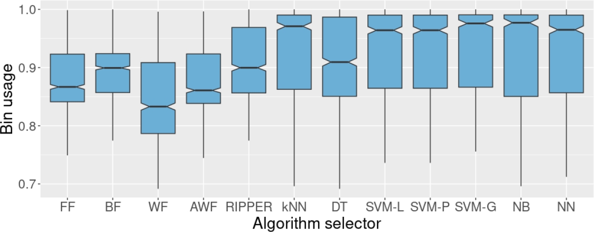
Fig. 5 Bin usage of the four heuristics and the algorithm selectors on the test set. These algorithm selectors were trained on set AX50. AX50 contains 50% of missing values in the individual results of the heuristics.
Training with 10% of missing values in the results of the heuristics seems to have little impact on the performance of the algorithm selectors produced. As in the case of the first experiment, the algorithm selectors produced in this experiment outperform the heuristics when compared in a pairwise manner, with 95% of confidence (the classifiers’ notches do not overlap with those of the heuristics). However, as the percentage of missing values increases, the performance of some algorithm selectors decreases.
For example, when 25% of the data about the heuristics is lost, RIPPER and kNN significantly reduce their performance, reaching only 41.5 and 50.3%, respectively (see Figure 4 and Table 1). However, regarding how they solve the instances, only RIPPER and DT are affected, reducing their performance close to the one of BF, the best individual performer of the heuristics. The remaining methods and the accuracies obtained are shown in Table 1.
When trained on AX50, a set containing 50% of missing values concerning the results of the heuristics, the performance decreases even more. This time, RIPPER and kNN correctly classify only 27.4% and 43.2% of the instances in the test set. However, when kNN fails to select the best heuristic, it fails selecting a competent heuristic, reducing the impact in its performance in terms of bin usage. According to the bin usage metric, RIPPER and DT fail as algorithm selectors since they somehow replicated the behavior of BF, the best individual heuristic in the test set according to its bin usage.
The algorithm selectors powered with SVM-G, Naïve Bayes Classifier and Neural Networks were capable of maintaining a solid performance even when 50% of the data regarding the heuristics was missing during the training process, obtaining an accuracy of 57.9%, 58.3%, and 59.4%. We provide the accuracy obtained by the remaining methods in Table 1.
Something worth mentioning is that the outliers disappeared when we used test set AX50. Contrary to what we might think at first sight, this is not a good indicator. The outliers disappeared because some methods exhibited a larger standard deviation in their results. Thus, the values that were considered unusual in previous cases are now considered ‘normal’ because the data are more spread out.
4.3 Working only with Complete Cases
The third experiment used a standard approach for handling missing values known as complete cases analysis. This involved removing any instance from the AX10, AX25, and AX50 datasets where at least one heuristic result was missing. As anticipated with this method, the number of training examples decreased proportionally to the number of missing values. Consequently, the resulting datasets —BX10, BX25, and BX50— experienced reductions of 33.9%, 68.3%, and 94.8% in the number of instances, respectively (see Figures 6, 7, and 8). That such a significant loss of data is impractical for real-world applications. Nonetheless, this experiment was designed to examine the effects of missing values and evaluate the impact of commonly used techniques for addressing them.

Fig. 6 Bin usage of the four heuristics and the algorithm selectors on the test set. These algorithm selectors were trained on set BX10. BX10 originally contained 10% of missing values in the individual results of the heuristics, but for this experiment, only complete cases were considered.
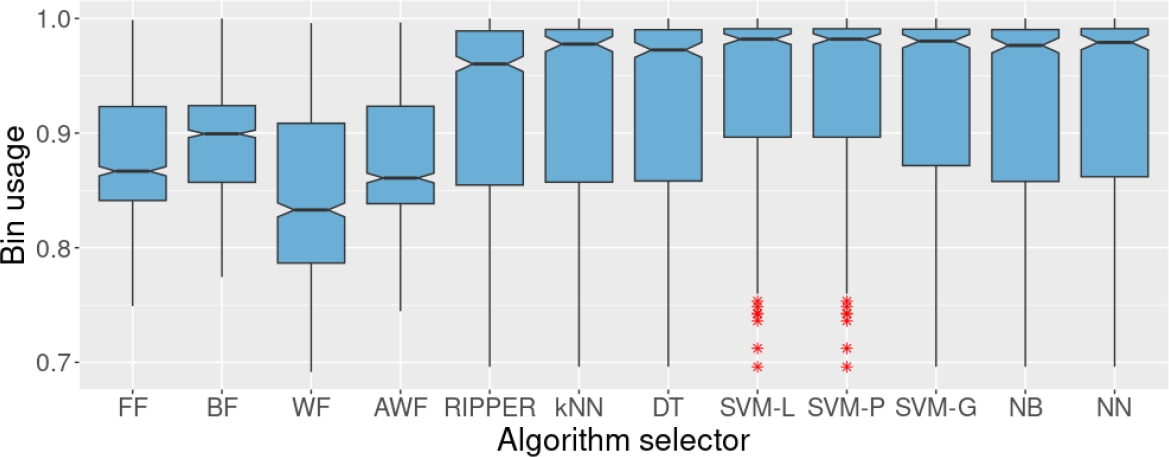
Fig. 7 Bin usage of the four heuristics and the algorithm selectors on the test set. These algorithm selectors were trained on set BX25. BX25 originally contained 25% of missing values in the individual results of the heuristics, but for this experiment, only complete cases were considered.
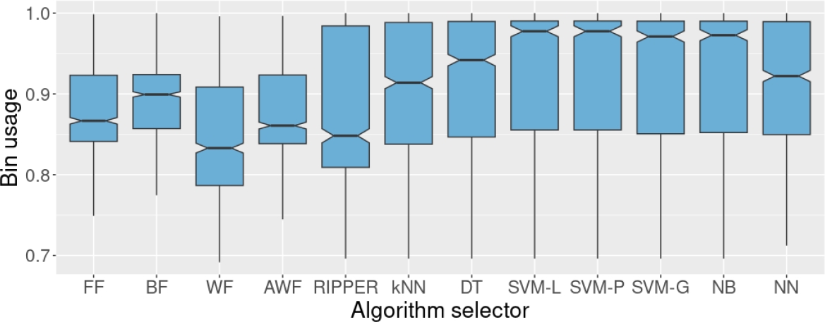
Fig. 8 Bin usage of the four heuristics and the algorithm selectors on the test set. These algorithm selectors were trained on set BX50. BX50 originally contained 50% of missing values in the individual results of the heuristics, but for this experiment, only complete cases were considered.
Similarly to what happened in the previous experiment, eight algorithm selectors were trained using the sets BX10, BX25, and BX50 to evaluate their performance on the test set. The rationale behind this experiment is to evaluate if keeping only complete cases may be used to deal with missing values in the context of algorithm selector generation.
When trained using only the complete cases (sets BX10, BX25, and BX50), the algorithm selectors did not exhibit an apparent decrease in performance regarding the bin usage, at least with sets BX10 and BX25 (which come from sets with 10% and 25% of missing values per heuristic). The algorithm selectors trained with BX10 are similar to those generated with TX00 and AX10.
What is more surprising is that the performance of RIPPER and kNN are better on the test set when trained on BX25 than on its counterpart, AX25. With these training sets, the algorithm selectors that showed the best performance in terms of accuracy were SVM-L, SVM-P, and NN, with 65.2%. Training on set BX25 decreased the performance of all the algorithm selectors (see Table 1). Despite that, some remained competitive and statistically superior to the other methods. That is the case for SVM-L, SVM-P, and SVM-G, which obtained an accuracy of 59.0%, 59.0%, and 56.2%, respectively. Conversely, RIPPER and kNN were severely affected by the drastic reduction in the number of examples for training when using set BX50.
4.4 Training with Data Imputation
For the final experiment, data imputation techniques were considered. Data imputation refers to a method for retaining the majority of the dataset’s data and information by substituting missing data with a different value. Thus, rather than retaining only complete cases, we synthetically generated values to fill the gaps in the AX10, AX25, and AX50 datasets. This process involved calculating the median bin usage per heuristic (excluding missing values) from the training set and using this median to impute any missing values for the heuristics. While this method enabled us to retain all records, it comes with a trade-off: some imputed values could potentially introduce bias in the selection of the optimal heuristic for each instance.
As depicted in Figure 9, training the algorithm selectors on set CX10 did not affect the performance of the selectors. In fact, the results obtained on the test set when training with AX10, BX10, and CX10 are almost identical. Then, 10% of missing values seem not to affect the training process. The decrease in the performance of some algorithm selectors, such as RIPPER and DT, is evident when we train using CX25 (Figure 10). Regardless of this reduction in the performance concerning bin usage, RIPPER remains statistically superior to the four heuristics (in a pairwise comparison) with 95% confidence (the notches of the boxplots do not overlap).

Fig. 9 Bin usage of the four heuristics and the algorithm selectors on the test set. We trained the algorithm selectors on set CX10. CX10 originally contained 10% of missing values in the individual results of the heuristics, but we replaced that 10% of missing values with the median of the corresponding heuristic.

Fig. 10 Bin usage of the four heuristics and the algorithm selectors on the test set. We trained the algorithm selectors on set CX25. CX25 originally contained 25% of missing values in the individual results of the heuristics, but we replaced that 25% of missing values with the median of the corresponding heuristic.
Finally, Figure 11 shows the worst scenario in this study, which occurs when CX50 is used to train the algorithm selectors and we can observe a significant decrease in the accuracy of almost all the selectors. In this case, the selectors are not statistically different from BF, the best individual heuristic on the test set. The only algorithm selectors that remain competitive under these conditions are NB and NN, which obtained accuracies of 57.1 and 41.5%. The rest of the results for this dataset are shown in Figure 1.
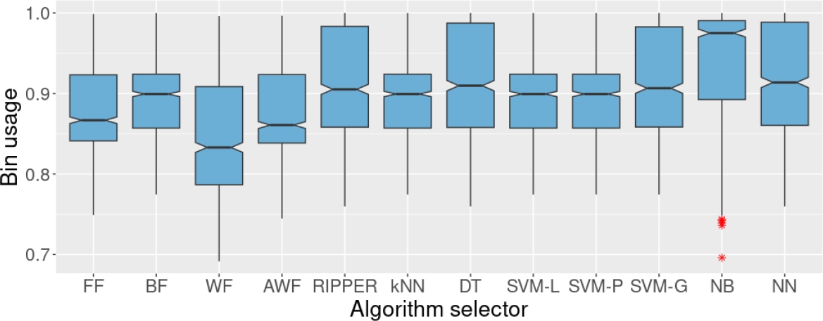
Fig. 11 Bin usage of the four heuristics and the algorithm selectors on the test set. We trained the algorithm selectors on set CX50. CX50 originally contained 50% of missing values in the individual results of the heuristics, but we replaced that 50% of missing values with the median of the corresponding heuristic.
5 Conclusion and Future Work
We have examined several scenarios involving missing values and their impact on the performance of algorithm selectors used as classifiers. Our findings indicate that missing values during training do not necessarily impair the performance of these algorithm selectors (see Table 1). This opens up the possibility of intentionally using missing values to reduce the computational resources needed for their generation.
For example, missing values could be introduced in the training data by systematically avoiding solving the training instances with some heuristics. Since we can control which cases to avoid solving, we can guarantee to keep a Missing Completely at Random (MCAR) scenario, which is the one where all the cases exhibit the same probability of being missing.
This idea could lead to important savings of up to 25% of the computing power devoted to solving the instances during the training process.
Besides, we observed that working with 10% and 25% of missing values does not seem to significantly change the methods’ general performance, regardless of whether they work with complete cases or use data imputation.
However, for larger proportions, such as 50% of missing values, the methods’ performance presents a notorious decrease, regardless of the technique used to deal with the missing values
Moreover, an interesting situation is yet to be explored: the occurrence of qualitative features to characterize the problem instances. So far, the work conducted on algorithm selectors for the BPP has relied on quantitative features only.
Although there is no apparent reason to think that the ideas presented in this work could not apply to such a scenario, we can only affirm that they will be useful once they have properly been tested.
Based on this investigation, we have identified several potential avenues for future research. While our current study focused on Missing Com-pletely at Random (MCAR) scenarios, exploring more complex cases such as Missing at Ran-dom (MAR) and Missing Not at Random (MNAR) could be valuable [11].

