


 nueva página del texto (beta)
 Inglés (pdf)
 Artículo en XML
 Referencias del artículo
 Enviar artículo por email
 Citado por SciELO
  Similares en
SciELO
Similares en
SciELO 
 Permalink
1 Introduction
Recently our work has been focused in analyze how the cochlea behavior can help to increase the recognition tasks for audio signals (speech recognition, music transcription; among others).
This research began with the study of the cochlea mechanical models with the objective to find which model or models could be used for our work. Undoubtedly, a great amount of works has been proposed at respect. After that, we analyzed a great quantity of paper and then we decided to use [1] and [2] for our research because of they represent one of the most important results and near to the functionality of the cochlea.
One time that the last cochlea models were selected the next challenge to reach was how to use these models to try to obtain o set of features or parameters that could be used in machine learning algorithms to obtain better results with respect to another proposed that are implemented actually.
For example, for speech recognition, MFCC parameters have been used for a long time. For another side, in music transcription algorithms such as NMF (Non-Negative Matrix Factorization) the Fast Fourier Transform (spectrogram) has been employed.
Specifically, NMF uses a spectral analysis of the audio signal based in Fourier Transform, obtaining spectrograms as the standard representation.
Independently that the task could be speech recognition or music transcription mentioned above its possible to modify the spectral representations with our propose based in the cochlea models. Along of this paper we show how to use these cochlea models to obtain audio signal parameters and how they can be applied to recognition tasks or to modify the spectral representations that are used in NMF algorithm.
This paper is organized as follows. Section 2 presents state of the art, in section 3 materials and methods are shown, while in section 4 the experiments are listed, finally conclusions and future works in section 5 are presented.
2 State of the Art
The development of cochlear mechanics analysis and modeling started during the 20th century. The first steps appeared around 1925, but the research was expanded strongly after 1950. The mathematical biophysical approach remained mostly linear until the late 1970’s, even though several nonlinear auditory phenomena were well known [3].
The initial study of the linear cochlea is relevant because of:
The first mechanical theory of the cochlea was proposed by Peterson and Bogert in 1950 [5]. It was based on hydrodynamics, considering the cochlea as a system of two channels that vary in shape, similar in cross section, and separated by an elastic membrane with constant dynamic variables. The model makes use of the parameters reported in the experimental work of Bèkèsy [4, 6]. In the following years, theories about the mechanics of the cochlea were developed, but in 1971 Rhode reported physical measurements of its physiology, and the theories that were proposed previously were found inadequate [7-8].
Later in 1972, Lesser and Berkley developed a model that matches all the previously reported observations, modeling the cochlea as a system with fluid flow, and the basilar membrane as a system of concatenated, forced, harmonic oscilators [1].
In 1976, Allen [9] used the Lesser and Berkley model to obtain the parameters of the basilar membrane using the Green’s function, obtaining an approximate set of parameters of its behavior. Later in 1981, Neely [10] proposed a two-dimensional mathematical model of the cochlea and their numerical solution using finite differences approximations of the Laplace’s equation, obtaining, so far and to the best of our knowledge, the best parameters of the mechanical response of the cochlea.
The solution to the model of the basilar membrane as a system of forced harmonic oscillators has been proposed by Lesser and Berkeley in 1972 [1], using potential flow theory and Fourier series. Later in 1974 [11], Siebert generalized the solution of Lesser and Berkley considering a mechanical force at the two ends of the basilar membrane. A similar solution was found in 1981 by Peskin [12].
The following studies considered the physical structure of the basilar membrane to solve the model, emphasizing studies in 1984 by Rhode [13], in 1985 by Hudspeth [14] and 1996 by Boer [15]. In recent years, authors have developed solutions considering state space models: in 2007 by Elliott et al. [16] and 2008 by Ku et al. [17]. Recently, these studies have been used for Automatic Speech Recognition Systems [18-19].
According to Place Theory of Hearing proposed by Helmholtz [20] and demonstrated by Békésy’s observations [21], the position along the basilar membrane at which the maximum hair cell and nerve response occurs is correlated with its frequency of the sound. Therefore, a function capable of calculating that relationship is called cochlear frequency-position function. From different methodologies for calculating these functions, Greenwood developed an accurate cochlear frequency-position function by integrating an exponential function fitted to a subset of critical bandwidths [22].
The critical bandwidth is the region along the basilar membrane where the nerve endings produce a large response to a sinusoidal audible signal. This is because the response of the hair cells along the basilar membrane to a sinusoidal tone is not limited to a single receptor or even to a narrow band of receptors, but to a bandwidth. For Music Transcription Tasks, we employed NMF (Non-Negative Matrix Factorization) as algorithm as is knowing this is a group of algorithms in multivariate analysis and linear algebra where a matrix V is factorized into (usually) two matrices W and H, with the property that all three matrices have no negative elements.
The way humans perceive music is related to their ability to identify signals coming from multiple separate sources. A transcription system performs a similar function by detecting notes from each individual source, classifying and grouping them into structures called dictionaries. An NMF model is capable of decomposing an input spectrogram as a part-based representation of sources or notes.
When applying the algorithm to the polyphonic TAM problem, the objective of the algorithm is to Factor a non-negative matrix:
a time-frequency representation of the signal with M ∈ ℕ as the feature dimensions and N ∈ ℕ as the number of segments over time, in two matrices [23]:
The range R ∈ ℕ is a constant parameter defined at the beginning of the algorithm; in the case of polyphonic.
TAM, it corresponds to the number of tones to recognize in the musical piece.
Works related and founded in the literature has shown that initializing W and H along with update rules can dramatically improve the chances of NMF converging to a musically favorable solution. Therefore, in the state of the art, when the STFT technique is used to generate the matrix V, it is recommended to initialize each of the elements of W with the Fourier magnitude spectra that in turn correspond to each of the notes of the instrument, for this work the piano.
For a long time, Automatic Speech Recognition Systems have used parameters related with Cepstrum and Homomorphic Analysis of Speech [24] Linear Prediction Coefficients (LPCs) [25], Mel Frequency Cepstrum Coefficients (MFCCs) [26], Perceptual Linear Prediction Coefficients (PLPs) [27], these last two being the most important.
This set of parameters uses spectral representation as the most significant representation of the speech signal. In each of these representations, the principal objective is to have a representation to compress the speech data without irrelevant information pertinent to the phonetic data analysis and to enhance aspects of the signal that contribute significantly to the detection of phonetic differences.
Other tasks where the reduction of the information of the speech signal is relevant are there when a great amount of reference information, such as speech signals for ASR that employed digital networks, is stored. Then, the reduction in the capacity of this information is a problem when we process database speech, used for transmission or storage [28, 29].
Undoubtedly, speech is the most important auditory information perceived by humans, but the auditory system does not respond as a linear but a logarithmic measurement system. MFCC and PLP coefficients employ Mel and Bark scales respectively that consider perceptual aspects to obtain a set of coefficients that rep- resent the speech signal.
One aspect to mention is that cochlea properties have not been considered. Inside the cochlea a particular frequency analysis is realized. It transforms frequency response into distance response [30]. Then, the solutions before mentioned take only the perceptual response without considering the principal operation of the cochlea. Therefore, to understand the cochlear operation using models permits an analysis of speech signal closer to hearing human.
3 Materials and Methods
One of the most important characteristics related with cochlear models is to try to find a response that can be adjusted to the cochlea behavior, in state of the art, it is possible to find the Greenwood’s work [31] that explain how the basilar membrane works when a frequency pulse is coming there.
Greenwood demonstrated his function fitted consistently cochlear observations on human cadaver ears and, with changes of constants, those on elephant, cow, guinea pig, rat, mouse, and chicken [31], as well as in vivo (behavioral-anatomical) data on cats. Twenty-nine years later, Greenwood used the same basic function and extended his study with observations in new physiological data of human, cat, guinea pig, chinchilla, monkey, and gerbil [31]. He proved the newer extended data were fit by the same basic function quite well (1):
where f is frequency (Hz), x is the distance from the apex of the cochlea (helicotrema end), A=165.4, a=0- 01, and k=1 are coefficients [31]. a is the gradient of high frequency end of the map, i.e., the coefficient of the derivative evaluated at the highest frequency, A is a constant which shifts the curve as a whole for a long the log-frequency axis, and k is constant, which introduces curvature into the frequency position function so as to fit low-frequency data.
The function essentially required only an empirical adjustment of a single parameter to set an upper frequency limit.
As Greenwood, Jimenez and Oropeza [19] also developed a methodology to obtain the relationship between the excitation frequency in the cochlea and the corresponding distance along of the cochlea but based on a different approach. Jimenez and Oropeza [19] found his function solving the model of fluid mechanics developed by Lesser [1] through an analysis of mechanical resonance:
where:
From (3) we can obtain the following expression to try to find the distance that depends of a specific frequency:
where (4) is a generic expression because of its possible to find different values of the
After that, to demonstrate that is possible to find a similar equation but using another cochlear model.
We used the model proposed by Neely in [10]. But now, using analysis based in non-linear regression to obtain the relation between frequency and distance, was used. The mathematical expressions obtained are the following:
This same equation is able to be expressed as the position along the cochlea as a function of frequency as (6) demonstrate:
With equations (2), (4) and (6), we are able to predict the position if maximum displacement on the basilar membrane as a function of frequency and vice versa. Figure 1 shows the pressure level with respect a frequency value such as Neely algorithm propose.
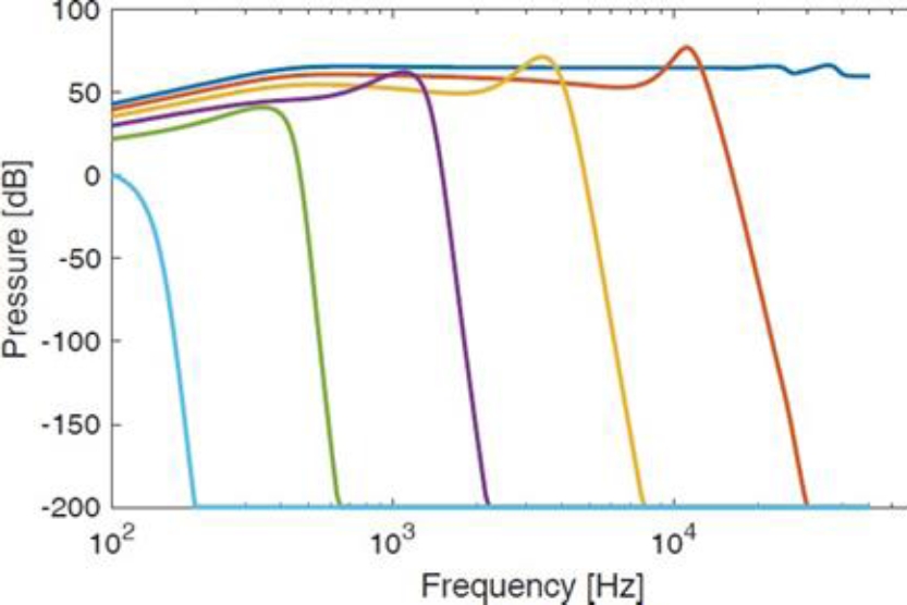
Independently of the cochlea model used, it must to try to adjust to the representation showed in fig 1. Then each one of the expressions (2) (4) and (6) determinate the distance where a frequency is present given the pressure difference in basilar membrane and where it has the most great value of excitation as is showed in figure 2.
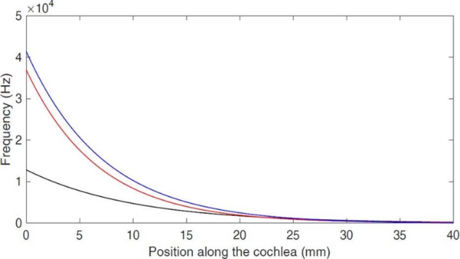
The result of curve obtained from the function (4) developed in this work is consistent with the curve of Greenwood’s function (2). On the other hand, the curve of function proposed by Jimenez used the following values k(x)=109e-2x, R(x)=200 and M(x)=0.15.
Figure 3 shows the diagram for the polyphonic music transcription using NMF algorithm. Our propose consists in add the spectral auditory-filtering block to modify the time/frequency representation (spectrogram of the signal) but using an auditory bank-filters, where central frequencies of each filter is obtained according to the equations (3,4,6).

4 Results and Discussions
In this section we compare and validate our propose join the Greenwood solution with respect to standard parameters or spectral representation used in ASR systems and Music Transcription respectively. As a first experiment, the frequency values for N = 251 points along a 40 mm long cochlear partition were calculated.
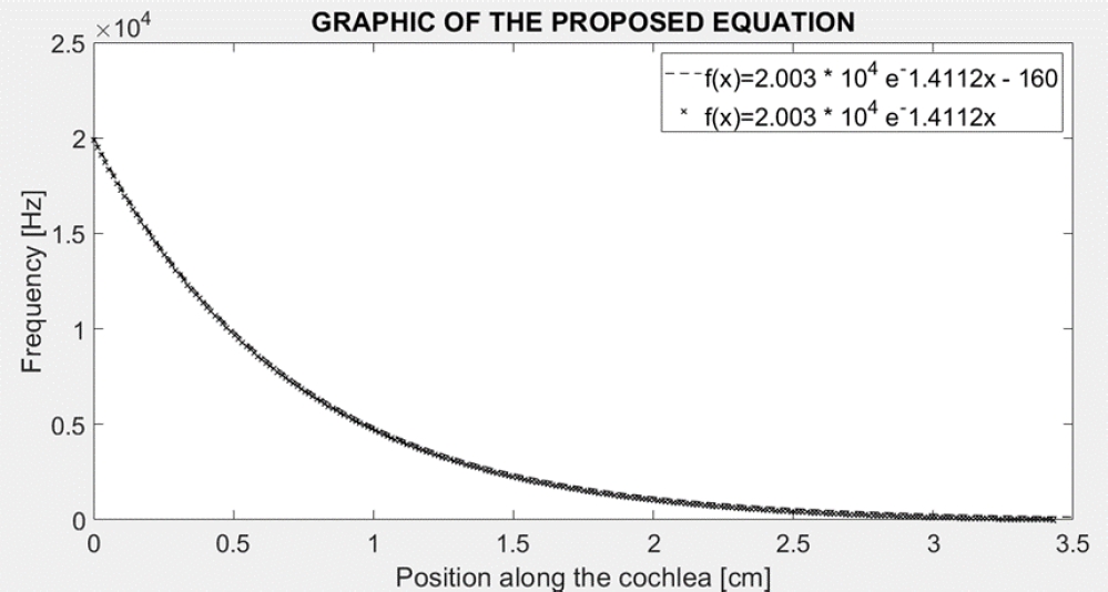
Figure 4 shows the behavior of the equation 5 when a factor k is plus to it.
One time that we find an equation that show the behavior of the cochlea related with the excitation frequency-distance is possible to apply it to different fields of the science.
For that, we selected two applications: Automatic Speech Recognition and Music Transcription, both of them associated with the human auditory. It is important to mention that each of them has its particularities and so much algorithms have been proposed to try to solve the problem inside of them.
4.1 Distribution of the Frequency Relationship with its Position along the Cochlea
As mentioned in the first section of this work, the cochlea behaves like a filter, which has a bandwidth bounded by a maximum frequency
From the last analysis a computational model to obtain the distance where the maximum displacement of the basilar membrane occurs to a specific excitation frequency of the system was developed, which depends of the physical characteristics of the basilar membrane.
The following procedure shows in table 1 describes the computational model of the cochlea using this propose [10]. It is important to mention that the maximum response of the pressure curve used in [10] was obtained.
Table 1 Description of the procedure to obtain MFCC coefficients modified
| → Obtain speech signal, realize preprocessing (It includes pre-emphasis, segmentation, windowing and feature extraction), for each sentence. → In the feature extraction, the same procedure as MFCC was used but the filter bank is constructed following the next steps. o Take the minimal and maximal frequency, where filter bank are going to be constructed. Default HTK uses o For each center frequencies of the bank-filter obtained with MFCC we must to obtain the distance in the cochlea from equations 4 or 6, it depends what kind of model we want to use. |
o Determine the linear frequency related with these distances, this represents the center of the filter bank using equations 1, 3 or 5. o Construct filter bank with frequency center obtained from the Mel equation. → Follow the same steps to obtain MFCC, multiply spectral representation from Fourier Transform with filter bank, calculate energy by bands using logarithm, and finally, apply discrete cosine transform. → Obtain a new set of coefficients for each speech signal. → Train the ASR and proceed with recognition task using the new parameters. |
As we can see table 1 shows the procedure to obtain a set of parameters to be applied in Automatic Speech Recognition using the classical MFCC parameters but modified using our propose previously mentioned.
4.2 Transcription Model
The first step consists of calculating the spectrogram of the music signal of the piece to be recognized and storing the modified spectrum for each segment such as explained in section 3 and it was illustrated in figure 3, storing it in the V matrix.
The columns of W should be labeled and initialized with the filtered spectrum of each complete isolated piano note.
Since an optimal detection threshold is sought to obtain the best transcription performance, different experiments were carried out by setting the threshold value on each row of H.
This is how it was determined that the threshold value that provides the most consistent results is of µ+ 1/2 σ of the set of all rows of H. The performance of the proposed system is compared with Marolt's SONIC [32]. Likewise, using the same dataset and calculating the central frequencies from the Greenwood function presented in the last experiment when implementing the filter bank, it becomes possible to make a comparison and evaluate which cochlear function helps to be better in transcription task.
7Its important to mention that the last stage of the transcription system called post-processing consists of representing the W and H factors as elements of tone and temporal activity, respectively. Each column of W then represents a tone and each row of H is associated with it, describing its onsets and duration. This is how the final product of this stage consists of tone events, with their onset and duration.
Therefore, it is possible to obtain a segment-level transcription that in turn can be compared with a MIDI file that serves as a reference. In the second experiment, a corpus elaborated by J. Hansen at the University of Colorado Boulder was used [33]. Only 9 speakers with ages ranging from 22 to 76 were used and we applied normal corpus not under Stress sentences contained into corpus.
The words were “brake, change, degree, destination, east, eight, eighty, enter, fifty, fix, freeze, gain, go, hello, help, histogram, hot, mark, nav, no, oh, on, out, point, six, south, stand, steer, strafe, ten, thirty, three, white, wide, & zero”. A total of 4,410 files of speech were processed. Finally, Tables 2 shows results when using our proposal (Cochlear Mechanics Cepstrum Coefficients – CMCC-) the best representations used in the state of the art and in the last experiment versus MFCC in SUSAS corpus, while table 3 shows the results of the Music Transcription task for a corpus described in the first column.
Table 2 Results obtained for automatic speech recognition task for SUSAS Corpus
| boston1 | ||||||||||
| SENTENCE | N | H | S | WORD | H | D | S | I | N | |
| HTK normal | 91.43 | 224 | 21 | 245 | 91.67 | 231 | 7 | 14 | 0 | 252 |
| Greenwood | 91.43 | 224 | 21 | 245 | 91.67 | 231 | 7 | 14 | 0 | 252 |
| Our purpose 1 | 91.43 | 224 | 21 | 245 | 91.67 | 231 | 7 | 14 | 0 | 252 |
| Our purpose 2 | 91.43 | 224 | 21 | 245 | 91.67 | 231 | 7 | 14 | 0 | 252 |
| boston2 | ||||||||||
| SENTENCE | N | H | S | WORD | H | D | S | I | N | |
| HTK normal | 95.51 | 234 | 11 | 245 | 95.63 | 241 | 7 | 4 | 0 | 252 |
| Greenwood | 95.51 | 234 | 11 | 245 | 95.63 | 241 | 7 | 4 | 0 | 252 |
| Our purpose 1 | 95.51 | 234 | 11 | 245 | 95.63 | 241 | 7 | 4 | 0 | 252 |
| Our purpose 2 | 95.92 | 235 | 10 | 245 | 96.03 | 242 | 7 | 3 | 0 | 252 |
| boston3 | ||||||||||
| SENTENCE | N | H | S | WORD | H | D | S | I | N | |
| HTK normal | 96.73 | 237 | 8 | 245 | 96.83 | 244 | 7 | 1 | 0 | 252 |
| Greenwood | 96.73 | 237 | 8 | 245 | 96.83 | 244 | 7 | 1 | 0 | 252 |
| Our purpose 1 | 96.73 | 237 | 8 | 245 | 96.83 | 244 | 7 | 1 | 0 | 252 |
| Our purpose 2 | 96.73 | 237 | 8 | 245 | 96.83 | 244 | 7 | 1 | 0 | 252 |
| general1 | ||||||||||
| SENTENCE | N | H | S | WORD | H | D | S | I | N | |
| HTK normal | 96.73 | 237 | 8 | 245 | 96.83 | 244 | 7 | 1 | 0 | 252 |
| Greenwood | 96.73 | 237 | 8 | 245 | 96.83 | 244 | 7 | 1 | 0 | 252 |
| Our purpose 1 | 96.73 | 237 | 8 | 245 | 96.83 | 244 | 7 | 1 | 0 | 252 |
| Our purpose 2 | 96.73 | 237 | 8 | 245 | 96.83 | 244 | 7 | 1 | 0 | 252 |
Table 3 Results obtained for Music Transcription Task
| Piece name | Our metrics | SONIC | ||||||
| Pr | Exh | Exh | F-Mea | Pr | Exh | Exh | F_Mea | |
| Schubert_Impromptu_Op._90_No._4_in_A-flat_major | 60.47 | 59.55 | 42.86 | 60.00 | 72.06 | 58.04 | 47.38 | 64.30 |
| Chopin_Prelude_Op._28_No._20_in_C_minor | 75.80 | 51.27 | 44.06 | 61.16 | 84.72 | 47.43 | 43.69 | 60.82 |
| Prelude_I_in_C_major_BWV_846 | 62.51 | 60.73 | 44.52 | 61.61 | 81.95 | 59.56 | 53.65 | 68.98 |
| Tchaikovsky_Swan_Lake | 71.52 | 55.74 | 45.61 | 62.65 | 88.36 | 55.39 | 51.62 | 68.09 |
| Grieg_Peer_Gynt_Morning | 72.88 | 55.39 | 45.93 | 62.95 | 85.95 | 47.66 | 44.21 | 61.31 |
| Clementi_Sonatina_Op._36_No._1 | 54.78 | 76.29 | 46.81 | 63.77 | 78.84 | 85.13 | 69.29 | 81.86 |
| Pachelbel_Canon_in_D_major | 66.78 | 61.90 | 47.33 | 64.25 | 89.29 | 63.61 | 59.10 | 74.29 |
| Satie_Gymnopedie_No._1 | 75.62 | 58.07 | 48.92 | 65.70 | 92.40 | 50.37 | 48.36 | 65.19 |
| Rebikov_Valse_Melancolique_Op._2_No._3 | 70.51 | 62.48 | 49.54 | 66.26 | 66.79 | 49.60 | 39.78 | 56.92 |
The results of these experiments confirm that the behavior of the proposed function is close to the Green- wood’s function. Moreover, taking into account that his function fitted cochlear observations on human cadaver ears quite well, and with changes of constants, those on ten different species.
Therefore, the function proposed in this work obtaining from a new approach achieves the same objective, which is to describe the behavior simulated of the human ear but using mechanical cochlear models.
In Automatic Speech Recognition the results showed that with this purpose it’s possible to find a better result that MFCC coefficients because two words were recognized adequately. In Music Transcription the results showed that it’s possible to modify the spectrum employed in NMF algorithm using a bank-filter adapted to our equations that present a relation between frequency and distance into cochlea.
Both experiments showed that is possible to integrate the purpose in these aspects related with human hearing and is necessary to probe in other applications to analyze the scope of the proposal.
In our days, so many papers related with deep learning algorithms use the spectrogram or MFCC parameters as input information to Recurrent Neural Networks (RNN), Long Short-Term Memory (LSTM) or Transformers Neural Networks (TNN) [34-37].
5 Conclusions
The main contribution of this paper is the formulation of a cochlear frequency-position function based on a biomechanical model and its applications for Automatic Speech Recogniton and Music Transcription. We have demonstrated that such function is consistent with Greenwood’s function.
In addition, this study leaves a methodology to find cochlear functions based on a non-linear regression method among others computational algorithms, applicable for any data set of a frequency type vs position inside of the cochlear position. Such cochlear functions are exponential and they represent a very simple mathematical expression.
On the other hand, although the proposed function was obtained from a cochlear model it is also possible to perform the reverse procedure [5]. That is, such cochlear functions might aid in the development of cochlear models.
For example, in recent papers, recurrent neural networks or transformers are used but the spectral representations (normally spectrogram or MFCC) are used. Then one of the possible future works that can be developed is modify the behavior of this spectral representations by the propose presented in this paper trough a bank-filters constructed from human hearing at we presented for the music transcription task and compare the results with or without the bank filters.
Then will be interesting to show these ideas modifying MFCC by CMCC for ASRs tasks and spectral representation of audio signal by the filter bank proposed in this paper.

