


 nueva página del texto (beta)
 Inglés (pdf)
 Artículo en XML
 Referencias del artículo
 Enviar artículo por email
 Citado por SciELO
  Similares en
SciELO
Similares en
SciELO 
 Permalink
1 Introduction
Photovoltaic (PV) technology has emerged as an excellent alternative for power generation due to its widespread availability, decreasing installation costs, and minimal environmental impact [9]. However, the operation of this technology requires continuous monitoring to guarantee good performance, efficiency, reliability, availability, and profitability [14].
Monitoring PV modules involves various methods, from manual inspection to measurement of electrical parameters, electroluminescence, and aerial thermography [16]. Among these, aerial thermography stands out as a particularly relevant technique.
By using thermal cameras mounted on unmanned aircraft systems, aerial thermography not only reduces inspection time but also proves to be a reliable and accurate tool for detecting faults in PV modules since a module in good condition will display a uniform thermal distribution.
In contrast, a defective module will manifest areas of heightened temperature that may not be readily discernible to the human eye [3, 4].
In the given context, the scientific community has worked on developing vision systems for the analysis of infrared images, also known as thermal images. The primary objective is to identify thermal distribution patterns that facilitate the classification of faults within the PV module.
Deep learning-based approaches, particularly Convolutional Neural Networks (CNNs), have been used as an effective alternative to address the fault classification problem of PV modules using thermal imaging, such as the work conducted by Akram et al. [1] and Hwang et al. [15]. These studies yielded an accuracy rate of over 93% in identifying faulty modules. However, the authors have utilized their own datasets in these works, which, unfortunately, are not public.
Currently, few public datasets exist for PV module fault classification. The most used public dataset with the largest number of labeled multiclass thermal images (20,000), is the one reported by Millendor et al. [11]. This dataset has been used for fault classification, for instance, the work of Alves et al. [2], which reported a classification accuracy of 78.85% using a custom CNN model.
Also, Le et al. [7] improved the classification by implementing an ensemble of CNNs, resulting in an accuracy of 85.9%. Subsequently, Korkmaz et al. [5] proposed the utilization of a multiscale CNN and data augmentation, resulting in an accuracy of 93.51% through the generation of augmented images during the train and test stages. In contrast, Pamungkas et al. [13] suggested combining two CNNs and then evaluating the model’s performance with and without data augmentation.
They obtained an accuracy of 96.65% with data augmentation and 65.9% without it, illustrating that data augmentation before partitioning into training and testing subsets leads to overfitting, resulting in elevated classification results that lack generalizability.
Although infrared image analysis is a valuable tool for PV fault classification, it presents challenges due to the lack of clear visual distinctions caused by low contrast, similar temperature patterns, and sensitivity to environmental factors [12].
Labeling a dataset of PV faults in thermal images poses difficulties even for experts, as thermal anomalies can be subtle and subject to interpretation.
Additionally, given the nature of some failures, it is common for a dataset to contain more examples of some failures than others, which may result in a dataset containing an unequal distribution of examples, with a larger representation of one type of failure over another.
This instance imbalance poses an additional challenge for classification algorithms. In this work, a study of the inherent complexity of the most widely used infrared images dataset for PV faults and its impact on accurate classification is presented.
Specifically, a methodology for analyzing and quantifying this complexity, particularly within the context of fault identification in PV modules, is described. The assessment of complexity involves the measurement of several criteria, including linearity, data imbalance, and dimensionality, among others. For experiments, six predefined scenarios have been established by splitting the dataset in different ways.
The complexity of each scenario is then analyzed through a data complexity calculation method. Some interesting results were found, and some recommendations were derived from our experimental results. The remainder of this work is organized as follows.
In Section 2, the used dataset as well as the proposed methodology for analyzing the complexity and the influence in faults classification is described. Section 3 shows and discusses the obtained results. Finally, the conclusions are presented in Section 4.
2 Data and Method
This section describes the dataset used. The proposed methodology for analyzing the complexity of the dataset and how it influences its classification is also explained.
2.1 Dataset
Datasets become vital resources for developing automated supervised learning systems, such as supervised classification systems. In particular, the dataset reported by Millendor et al. [11] is one of the most used datasets for photovoltaic fault classification based on infrared images. This dataset comprises 20,000 infrared images with dimensions of 24 × 40 pixels.
These images were obtained by unmanned aerial vehicles equipped with medium and long wave (3 to 13.5 µm) infrared cameras. Image resolution varies from 3.0 to 15.0 cm/pixel. Each dataset image only showcases photovoltaic modules. Additionally, the dataset encompasses 12 classes, including 11 different types of failures, eight electrical and three environmental, and one non-anomaly class.
It is important to emphasize that within the context of PV fault detection systems, electrical faults take priority over environmental for a few key reasons. Primarily, electrical faults directly impact the efficiency and functionality of the PV module. For instance, hot spots resulting from malfunctioning components or improper connections can notably diminish power output.
In contrast, even though environmental factors may influence the overall thermal signature, these faults do not induce permanent damage. Then, this study is centered on classifying electrical faults through infrared analysis and their associated complexities. Fig. 1 shows the distribution of images by class of the electrical faults present in this dataset.
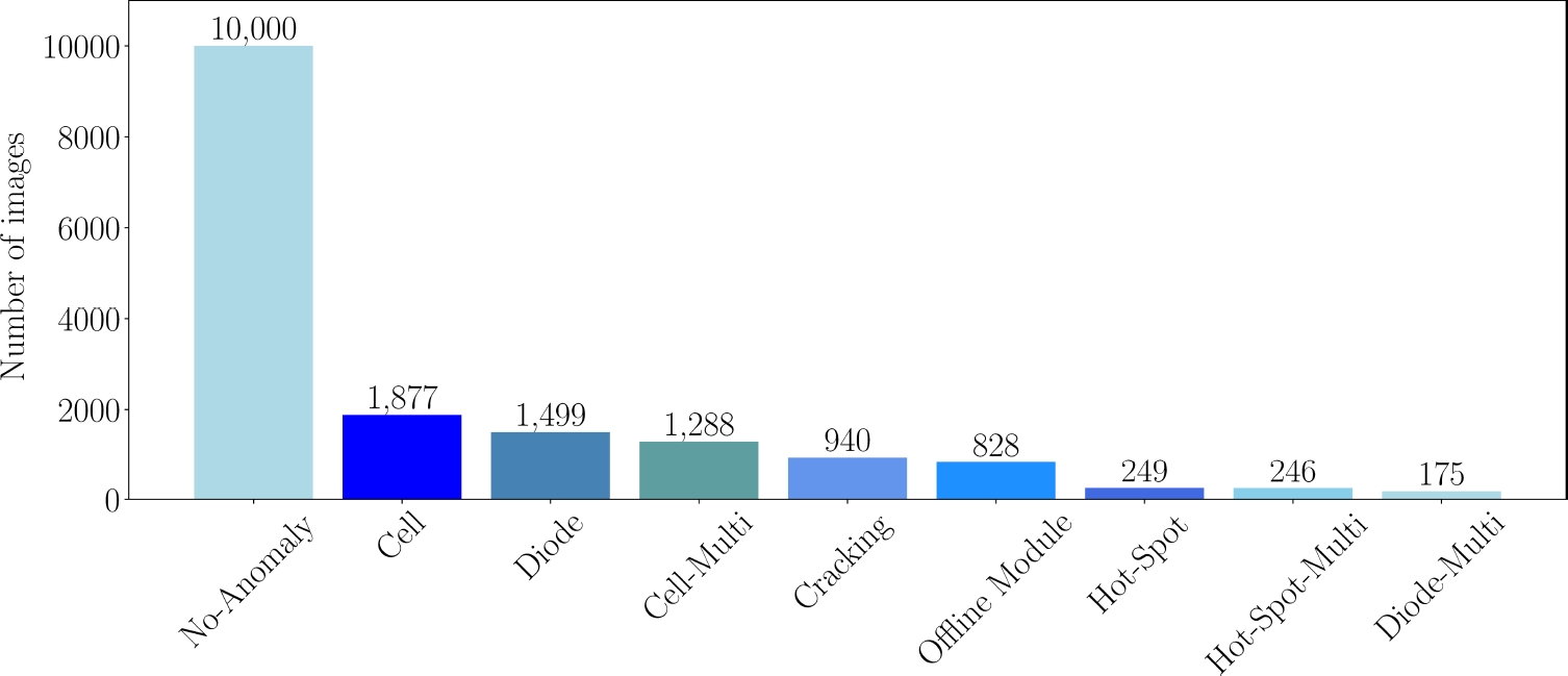
As it may be observed, the No-Anomaly class has the most instances, with 10,000 samples. From Fig. 1, it may also be observed that there is a significant imbalance in the number of class instances, with multiple by-pass diodes (Diode-Multi) having the fewest instances, with 175 samples. This imbalance can affect the perception of predominant patterns and features.
Fig. 2 shows the characteristic patterns of each type of electrical fault analyzed in this work. From a visual analysis, it may be possible to identify similarities within certain classes, as in the case of the cracking and multiple hotspot classes, which may share patterns that include multiple white spots.
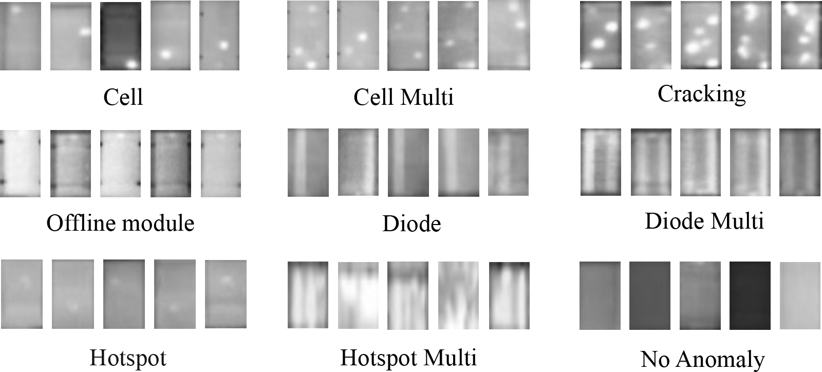
Fig. 2 Representative and visually differentiable images of each type of electrical faults present in the dataset [11]
To analyze how complex the dataset is, the images were encoded into feature vectors. These feature vectors were extracted from the images using the well-known CNN architecture AlexNet [6].
The AlexNet model has been chosen because it efficiently balances performance and computational requirements, enabling robust feature extraction without demanding excessive resources. Furthermore, its architecture facilitates both implementation and optimization.
The feature vector extraction process involved removing the final layers of AlexNet, specifically the classification part, leaving only the essential feature extraction functionality. The diagram in Fig. 3 shows the AlexNet architecture, highlighting the feature extraction and classification components.
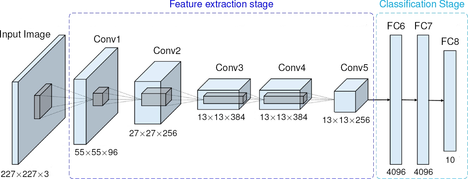
Fig. 3 AlexNet architecture structure. This CNN architecture is made up of five convolutional layers (Conv1 to 5) to extract features and three fully connected layers (FC6 to 8) for classification
Furthermore, to “visualize” the dataset complexity, the Uniform Manifold Approximation and Projection (UMAP) method [10] was employed. UMAP is a dimensionality reduction method suitable for nonlinear data. This approach primarily shows a low-dimensional visual representation of the distribution of the feature vectors.
2.2 Complexity Analysis
In the context of supervised learning tasks, data complexity denotes the inherent challenge posed by a dataset in terms of enabling a model to discern the underlying patterns [17].
This challenge may stem from high dimensionality, imbalanced classes, or noisy labels. Particularly in classification, assessing data complexity through various measures allows for estimating the difficulty involved in segregating data into specific and predefined classes.
In this work, six experimental cases (named Case I to VI) have been designed to assess the dataset’s complexity. Case I, serving as the baseline, involves the human expert’s manual selection of representative images from each category of electrical faults.
These images are chosen based on clearly identifiable class characteristics. Specifically, only 50 images from each class can be unambiguously identified as belonging to one and only one class. In Cases II and III, the number of images with respect to Case I has been augmented.
Specifically, in Case II, the number of images is less than in Case III; however, both cases have the same number of images per class, which means no data imbalance is found in them. This data balance is maintained until the number of images in the minority class (175 images) is reached.
As a result, Case II has 113 images per class, while Case III contains 175 images per class. In cases IV to VI, the remaining images of each class were uniformly and randomly sampled and subsequently added to the already selected images. In particular, a third of the total remaining images were added for each case.
If
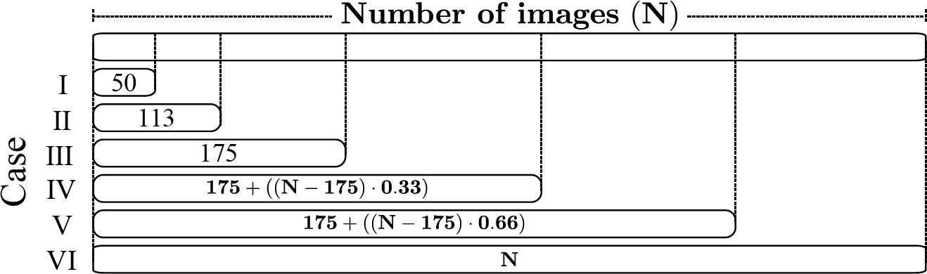
To illustrate, consider the “Cell” class, which initially comprised N=1,877 images. In Case I, 50 representative images of the “Cell” class were selected. In Case II, 63 additional randomly selected images were added to the Case I images.
In Case III, 62 more images, also randomly selected, were incorporated to reach the limit of minority class images. Note that in Case III, 175 images were already selected, leaving 1,702 (N-175) images for addition. These 1,702 images were then divided into three parts: two sets of 562 images each and one set of 578.
Consequently, for Case IV, 562 ((N-175)· 0.33) images were combined with the 175 images from Case III; therefore, Case IV will have a total of 737 images (175+(N-175)· 0.33). For Case V, an additional 562 images were included; then, the resulting number of images is 1,299 ((175+(N-175)· 0.66)).
Finally, for Case VI, the remaining 578 images were incorporated. The augmentation process is executed for each class. Note that, for cases IV to VI, the number of images augmented by classes differs due to the initial dataset imbalance despite the consistent proportion of images used.
To evaluate the complexity of each dataset’s case, the set of six complexity categories proposed by Lorena et al. [8] is used. The description of each category is the following:
– Feature-based. Assesses the discriminative capability of features in a classification task by employing metrics such as the Maximum Fisher’s Discriminant Ratio, the vector of the Fisher Discriminant Ratio, the volume of overlapping regions, and the efficiency of individual and collective features.
– Linearity. Evaluate the level of the problem to separate the classes by a hyperplane employing a Linear Support Vector Machine classifier.
– Neighborhood. Examine the decision boundary and analyze local neighborhoods of the data points by employing a fraction of the borderline point, the ratio of intra/extra class, error rate, and non-linearity of the Nearest Neighborhood classifier.
– Network. This category considers the instances as the vertices of the graph and evaluates its relations employing the density, clustering coefficient, and Hubs metrics.
– Class Imbalance. Evaluates the dataset based on the degree of data imbalance using the entropy of class proportions and the imbalance ratio.
– Dimensionality. Analyze the relation between the number of features and the number of instances in the dataset. Employing the average number of features per dimension, the Average number of Principal component analysis (PCA) dimensions per point, and the ratio of the PCA dimension to the original dimension.
It is pertinent to highlight that each category encompasses various “metrics”. Nonetheless, an average value derived from these metrics adequately conveys the level of complexity associated with each category.
2.3 Classification Performance
For the purpose of illustrating the impact of complexity on the classification task using a CNN, the AlexNet architecture was trained and tested with subsets from each of the six proposed cases. It is worth mentioning that this architecture has been retrained from the model that was previously trained on the ImageNet dataset [6]. Additionally, in all six cases, a 5-fold cross-validation is implemented during the training model stage to assess how well the model performs on unseen data. Furthermore, for all six cases, the best-performing model from the 5-fold cross-validation was tested on the test subset. The overall performance of the models has been evaluated using the classical metrics: Accuracy, Precision, Recall, and F1-score [18].
3 Results
In this section, the results of the complexity analysis, as well as the model classification performance, are shown. The implementation was carried out in Python 3.8 and PyTorch framework 1.13.1. In all six cases, the AlexNet model was trained using the Adam optimizer on 60 epochs with a learning rate of 0.00005, a batch size of 32, and categorical cross-entropy as a loss function. All the parameter values were set experimentally.
3.1 Complexity Analysis Results
A low-dimensional data projection is used to first approach the dataset’s complex analysis. As described in Section 2.1, this projection is implemented using the UMAP method [10].
This method tries to preserve the high-dimensional topological structure in a low-dimensional representation, which proves beneficial in evaluating data complexity, particularly in terms of class separability.
Then, to qualitatively evaluate the dataset complexity as the amount of information increases, the feature vectors of Case I (base case), Case IV (first unbalanced case), and Case VI (fully dataset) have been projected into a low dimensional representation. These projections are depicted in Fig. 5.
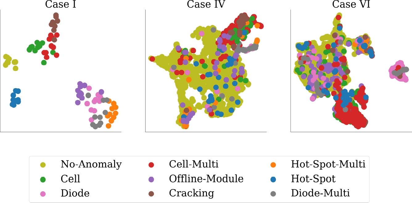
As it may be observed, in Case I, the feature vector projections unambiguously delineate “clusters”, exhibiting a spatial data distribution that implies a distinct separation between the groups. Conversely, discerning a clear separation of the data pertaining to the nine different classes in Cases IV and VI is visually challenging.
However, although qualitative analysis provides valuable insights into the relationship between complexity and the number of instances, the establishment of a series of quantifiable values is preferable for a more precise understanding of complexity. Thus, as previously mentioned, multiple categories have been implemented to measure complexity from various perspectives.
Table 1 shows the values from all categories from the six cases of study. As may be observed, Feature-based, Linearity, Neighborhood, Network, and Class imbalance categories have been grouped together. This is because the mean values of these categories range from 0 to 1, signifying that lower values indicate lower complexity while higher values suggest higher complexity.
Table 1 Mean values of complexity categories
| Case | ||||||
| I | II | III | IV | V | VI | |
| Feature-based | 0.017 | 0.102 | 0.138 | 0.171 | 0.173 | 0.191 |
| Linearity | 0.000 | 0.000 | 0.000 | 0.000 | 0.000 | 0.000 |
| Neighborhood | 0.306 | 0.399 | 0.414 | 0.406 | 0.400 | 0.404 |
| Network | 0.804 | 0.896 | 0.930 | 0.879 | 0.911 | 0.897 |
| Class imbalance | 0.000 | 0.000 | 0.000 | 0.313 | 0.393 | 0.395 |
| Average | 0.2255 | 0.2796 | 0.2963 | 0.3536 | 0.3753 | 0.3774 |
| Dimensionality | 17.329 | 7.867 | 5.130 | 3.344 | 2.560 | 1.276 |
However, it should be noted that the “Dimensionality” category does not conform to this range. From Table 1 may be observed, as expected, that Case I exhibited the lowest average complexity. Furthermore, it is noteworthy that all cases can be linearly separated, as indicated by the minimal complexity value in the “Linearity” category.
Conversely, a higher complexity value was observed across all cases when evaluating the Network category, suggesting a lack of structural information for graph modeling within the dataset.
On the other hand, considering that a classification problem is also addressed, the “Feature-based”, “Neighborhood”, and “Class imbalance” categories become relevant. Notably, under the “Feature-based” category, relatively low complexity values are observed, suggesting that the features of the classes may exhibit sufficient distinctiveness. Nevertheless, within the “Neighborhood” category, defining clear data separation becomes increasingly challenging as the data sets become denser.
Conversely, and as expected, for the “Class imbalance” category, Cases I, II, and III, cases with the same number of instances per class, an imbalance value of 0 is obtained, whereas for Cases IV, V, and VI, where a significant imbalance in the data is presented, a values of 0.313, 0.393, and 0.395, respectively, were observed.
Regarding the “Dimensionality” category, where the number of features concerning the number of instances is analyzed, it was observed that a higher value is attained when there are only a few instances.
In contrast, the dimensionality value decreases as the data volume increases. Consequently, Case I is the most complex under this category, whereas Case VI is the least complex.
3.2 Classification Results of Each Study Case
Data complexity and classification tasks are intricately linked. Complex data may significantly challenge the ability of a classification model to distinguish between classes accurately. Then, to analyze this relation, the best AlexNet model obtained by 5-folds cross validation on the test subset for each case is used. In Table 2, the classification results are shown.
Table 2 Classification results of each case
| Case | ||||||
| I | II | III | IV | V | VI | |
| Accuracy | 0.980 | 0.720 | 0.730 | 0.940 | 0.930 | 0.880 |
| Precision | 0.978 | 0.727 | 0.727 | 0.743 | 0.774 | 0.783 |
| Recall | 0.978 | 0.721 | 0.727 | 0.676 | 0.710 | 0.753 |
| F1-score | 0.978 | 0.718 | 0.722 | 0.703 | 0.733 | 0.766 |
| Number of images | 90 | 204 | 315 | 1351 | 2387 | 3420 |
In particular, in Case I, the best results in terms of Accuracy, Precision, Recall, and F1-score, with values of 0.98, 0.978, 0.978, and 0.978, respectively, are obtained. In contrast, the case with the worst results was Case II, with values below 0.73 in all metrics.
For Cases IV, V, and VI, high accuracy values above 0.88 were reached. This success was attributed to the model’s proficiency in accurately discerning the “No anomaly” class, which comprises a substantial number of instances compared to the other classes. However, considering the presence of an unbalanced dataset in Cases IV, V, and VI, it is advisable to focus on the F1-score metrics rather than accuracy.
F1-score provides a better reflection of model performance when dealing with unbalanced datasets. Then, in Cases IV to VI results lower than 0.79 were obtained for F1-score. From the obtained results, it can be concluded that adding non-representative class images in Cases II and III has a greater impact on the classification since the number of images is lower. In addition, adding non-representative images to a large number of instances, which additionally has an easily distinguishable class such as the “No anomaly” class, may bias the results, generating apparently better results as in Cases IV, V, and VI.
Another way to visualize the impact of dataset complexity on the classification task involves observing how often a trained model accurately classifies or confuses a never-before-seen input data, in this case, an image.
Confusion matrices, a “matrix” that organizes and shows the number of correct and incorrect predictions for each class, can be used to perform this visualization. By analyzing the confusion matrices shown in Fig. 6, the classes that are complex to differentiate from each other can be identified. As may be observed, the CNN model in Case I demonstrates a high capability to classify most data.
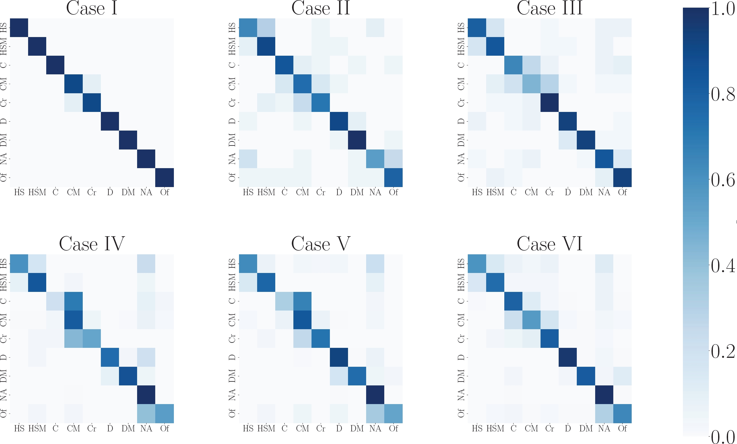
Fig. 6 Confusion matrices from Case I to VI. The classes are defined as HS: Hotspot, HSM: Multiple Hotspot, C: Cell, CM: Multiple cells, Cr: Cracking, D: Diode by pass, DM: Multiple Diode By-pass, NA: No anomaly, and Of: Offline module
This outcome is consistent with the results obtained in the complex analysis, in which Case I registers as the least complex case. In contrast, in cases II and III, where the datasets remain balanced, the model begins to encounter challenges with classification.
Conversely, a higher frequency of misclassified instances in cases IV, V, and VI looks evident. Nevertheless, despite Case VI being the most complex based on complexity assessments, its corresponding confusion matrix indicates superior model performance compared to cases IV and V.
This behavior may be attributed to a larger volume of instances available for training, potentially facilitating more effective weight adjustments within the convolution layers and, consequently, improved feature extraction capabilities. Nonetheless, regardless of the case study, several classes are hard to differentiate due to the image characteristics, making them more complex to classify.
For instance, “Cracking” and “Multiple cells” faults are the most difficult to differentiate in all cases. Furthermore, the presence of classes characterized by highly similar patterns, such as “cell” and “multiple cells”, as well as “hotspots” and “multiple hotspots”, presents another notable issue.
4 Conclusions
In this work, a study of the inherent complexity of the most widely used infrared image dataset for PV faults and its impact on the fault classification task has been presented. From the study, it is concluded that the complexity of the dataset is related to the quality of the data.
Particularly, based on the complexity analysis factor, such as the balance of the class instances, the linearity of the data, and the representativeness of the instances must be taken into account mainly to perform tasks such as classification.
Therefore, it is recommended that the complexity of the training data be analyzed before proposing solutions for classification tasks. In future work, the generation of a high-quality solar module dataset will be considered.

