


 nueva página del texto (beta)
 Inglés (pdf)
 Artículo en XML
 Referencias del artículo
 Enviar artículo por email
 Citado por SciELO
  Similares en
SciELO
Similares en
SciELO 
 Permalink
1 Introduction
The objective of Atmospheric Correction (AC) is to eliminate the effects of the atmosphere on satellite images to obtain the spectral characteristics of the surface. The atmosphere affects the light passing through it primarily in two ways, light scattering and absorption [1, 2].
The dominant atmospheric effect is scattering which is additive to the remotely sensed signals while multiplicative effect is caused by light absorption [3]. The main factors that distort satellite signals from the Earth's surface are aerosols and molecular scattering, as well as absorption by gases and particles suspended in the atmosphere [1, 2].
All gaseous and aerosol components of the atmosphere generate a distortion in the electromagnetic spectrum that causes the reflectance captured by the satellite sensors to include distortions that must be corrected to make a correct identification of the real reflectance values on the Earth's surface.
Over time, different methods have been developed to obtain the real reflectance of the Earth's surface, most of them are based on the theory of radiative transfer developed and published in 1960 by Chandrasekhar [4]. Some methods are based only on the image itself (i.e. Image Based), among which we have some such as DOS (Dark Object Subtraction) QUAC among others [1, 5, 6].
Others require auxiliary atmospheric parameters (i.e. FLAASH, 6S) [1, 5, 6], generally these methods are based on some radiative transfer code. Radiative transfer codes (RTC) are scientific software that numerically simulate the propagation of electromagnetic radiation through a medium. RT simulations are used in various disciplines, including astrophysics, Earth and planetary sciences, and Remote Sensing.
The most accurate methods have generally been those based on Radiative Transfer Codes (i.e., 6S, MODTRAN) [5]. However, the complexity, high dimensionality, and computational cost of numerical RTCs, particularly in large areas with large data sets, restrict their use in real remote sensing applications, including atmospheric correction. Traditionally, to overcome these problems, look-up tables (LUT: Look-up Tables) [7, 8] have been used to approximate the simulations of a radiative transfer code and recently it has been suggested to approximate numerical RTCs through machine learning, this approximation being known as emulation [9, 10, 11].
Machine learning (ML) algorithms, such as neural networks (Deep Learning), have demonstrated a good ability to emulate these complex and non-linear RTCs based on numerical methods. 6S RTC simulations have a simulation time of typically 0.97 seconds [12], while the emulation reduces the computation time.
In this work, we propose and compare four different architectures based on Deep Learning (DL) to emulate a 6S radiative transfer code. In this approach, instead of using LUTs (Look-Up Tables), TOA (Top of Atmosphere) values along with a subset of other atmospheric parameters are used by DL models to predict the correct SR (Surface Reflectance) values [13].
The database was created from synthetic data generated using simulations in the RTC 6S, in particular the development was done using the Python interface with 6S called Py6S, developed by [14,15].
2 Theoretical Background
This section presents the main ideas and procedures used in the construction of a synthetic data set and the analyzed models. It includes brief descriptions of the RTC used (6S) as well as the models used in this comparison.
2.1 Atmospheric RTC 6S
The Second Simulation of the Satellite Signal in the Solar Spectrum (known, understandably, as 6S) is a Radiative Transfer Model that is widely used in remote sensing. It simulates the effect of the atmosphere on the light passing through it.
6S was originally developed by a team led by Eric Vermote and is described in detail in [16] and the original manuals. The original objective of this RTC was to describe the effects of the dispersion and absorption of atmospheric gases and aerosols on the propagation of solar radiation both downward and upward through the atmosphere, taking into account that sunlight passes through when the atmosphere reaches the Earth, it interacts with the Earth's surface and returns to the atmosphere where it passes through it again and is captured by the sensors in space.
The 6S code can be used on two types of surfaces:
– Isotropic (also known as Lambertian), in which a diffuse reflection occurs. For this study it is assumed that the surface is Lambertian, which offers acceptable results in most cases, except when the value of the optical thickness of the aerosols is high [17].
– Anisotropic. A classic example of an anisotropic surface is water, since the reflection of light is not homogeneous but specular, that is, it depends on the angle of incidence of the light and the angle of view of the observer (i.e., BRDF).
2.2 Deep Learning
Deep Learning (DL) is a branch of Artificial Intelligence that belongs to the techniques of so-called Machine Learning. It gained particular importance in the early 2010’s mainly due to the use of convolutional neural networks (CNN) in computer vision applications [18].
Since then and due to the good results, that these algorithms have given, the use of these networks has been extended to other applications such as language (Natural Language Processing), audio, video, etc. Regression problems commonly solved with DL models consist of predicting the value of a continuous variable from certain input.
Because of this, continuous variables such as reflectance can be estimated using a DL model to predict their value, so the model is trained to do regression using different combinations of input parameters and using the data obtained through simulations, in this case simulations with the RTC 6S.
DL models need a loss function, which is the one that will be optimized during model training. For regression problems, the commonly used loss function is the so-called MSE (Mean Squared Error). In this work we present 4 models that are suitable for regression such as MLP, 1D-CNN, MLP-NE (Multilayer Perceptron with Numerical Embedding) and an architecture based on the ViT (Vision Transformer).
2.2.1 Multilayer Perceptron (MLP)
The multilayer perceptron is an artificial neural network formed by multiple layers (generally dense layers, that is, fully connected layers), usually an input layer, intermediate layers also called hidden layers and an output layer. Each neuron usually contains an activation function that introduces nonlinearity into the network. One of the most used activation functions is ReLu. MLPs have been used in atmospheric correction and aerosol optical thickness (AOD) estimation applications [19, 20, 21, 22].
2.2.2 One Dimension Convolutional Neural Networks (1D-CNN)
Traditionally convolutional neural networks have been used for images, hence two-dimensional filters (kernels) are used. In reality, the kernel can be of any dimension, which is why its use has spread in applications that require one-dimensional kernels such as text, audio, etc. Recently, the use of 1D-CNN has been proposed to estimate bidirectional reflectance in satellite images [9].
These networks consist of convolutional layers (to extract features), Maxpooling layer (to reduce dimensionality of the data) and a classification or regression layer made up of dense layers.
2.2.3 Multilayer Perceptron with Numerical Embedding (MLP-NE)
Recently improvements have been made to the performance of the MLP, using what is known as numerical embedding. “Embedding” is a vector representation of some parameter.
The concept comes from the area of Natural Language Processing in which a word is represented as a vector. In the article “On Embeddings for Numerical Features in Tabular Deep Learning” [23], the authors demonstrate how the vector representation of scalar parameters can substantially improve the performance of MLP in applications with tabular data (i.e. they have categorical and numerical data).
One of the ways to do numerical embedding that is presented in this work is to do a dimensional expansion of each parameter using a dense layer [24]. In this work, “Numerical Embedding” is used to represent each input parameter as a vector, so that the input to the MLP is no longer a set of scalar data, but a set of vectors.
2.2.4 Vision Transformer (ViT)
The original Transformer was designed to be used in Natural Language Processing applications, later in 2021 it was extended to be used in computer vision applications. The idea of the Vision Transformer (ViT) is to decompose the image into “patches” and convert each patch into a vector, treating it as if it were a word [25].
In this work, an architecture based on the “Vision Transformer” is proposed that incorporates “Numerical Embedding” to represent each parameter of the input model as a vector so that the ViT processes a sequence of parameters represented as vectors, that is, the matrix of embeddings is made up of a set of vectors in which each vector represents a scalar parameter, where each input parameter is numerically embedded (vectorized) to form the embedding matrix.
Table 1 Description and ranges of the 6S model key input parameters used to simulate Surface Reflectance
| Parameters | Symbol | Description | Unit | Range | Step |
| Sun-Sensor Geometry | SZA | Sun Zenith Angle | Deg | 40-70 | 10 |
| VZA | View Zenith Angle | Deg | 0 (Nadir) | N/A | |
| SAA | Sun Azimuth Angle | Deg | 120-240 | 40 | |
| VAA | View Azimuth Angle | Deg | 120-240 | 40 | |
| Atmospheric Optical | AOD | Aerosol Optical Depth | Unitless | 0-0.5 | 0.1 |
| Atmospheric Model | N/A | Midlatitude Summer | Unitless | N/A | N/A |
| Aerosol Model | N/A | Continental | Unitless | N/A | N/A |
| Radiance | RAD | Apparent Radiance | 0-450 | 50 |
Unlike the original ViT, in this proposal “Positional Embedding” is not used since the position of the parameters is not relevant, as is the position of the patches in an image.
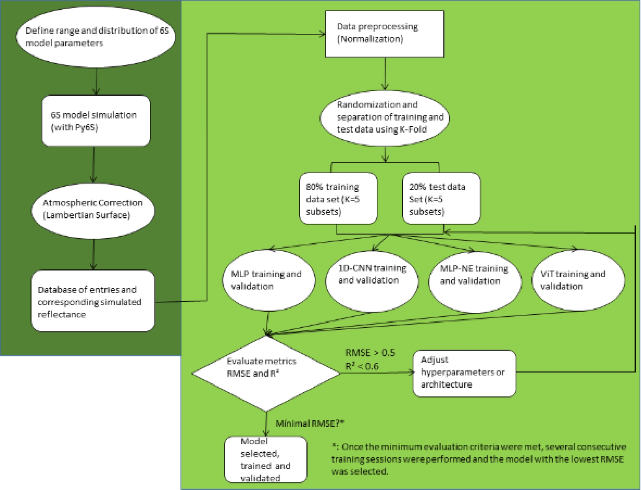
3 Material and Methodology
The methodology proposed in this article is divided into 2 phases. The first phase consists of doing enough simulations with Py6S (3840 simulations were carried out) with different values for the sun-satellite geometry, different atmospheric conditions and different radiances captured by the satellite sensor according to the range found in the metadata file.
Subsequently, random samples of 80% of the total data were generated to create the training data set of the models, the remaining 20% was used to create the validation data set with which each model was tested [9, 22]. The second phase consists of training and validating the four model architectures presented in the previous section.
Validation is done with respect to two metrics that are the root mean square error (RMSE) and the coefficient of determination (R²). Additionally, the inputs were normalized using the “Min-Max Normalization” method.
In general, the optimization of all hyperparameters was carried out iteratively until the combination of parameters that offered the best results was found. In general, there is no fixed methodology to find the best values for the hyperparameters in this type of applications [22] since the “optimal” value of these depends on many factors.
3.1 Parameter Range for Generating Synthetic Data with the RTC 6S
To create the data set with which the models will be trained, a series of combinations of different variables were created within a previously defined range that adjusted to the typical values of the area of interest being worked on.
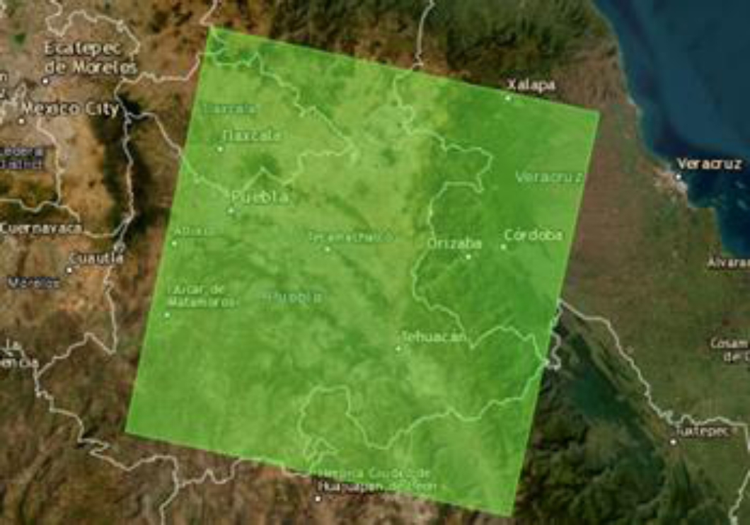
This area of interest is located in scene WRS 25/47 which covers the states of Tlaxcala, Puebla, Veracruz, Oaxaca and a small portion of the state of Hidalgo.
The following figure shows the footprint of scene WRS 25/47. Although it is not a critical parameter used in simulations carried out with 6S, when making atmospheric corrections, it is recommended that the percentage of cloud cover (Land Cloud Cover) be less than 10% although NASA recommends using images of up to 20% with cloud cover, it also depends on the area studied, some researchers suggest no more than 20%, so 10-20% is usually an appropriate value to be selectedfn. However, to make land use classification for example, the percentage can be even lower 5-6% [26].
The ranges of the variables used are the following: Additionally, one of the images of this area captured in month 5, day 16 was selected since the translational movement of the earth is also taken into account when making the simulation and finally the “Coastal/Aerosol” band was selected, whose Central wavelength value is 442.96nm (obtained from Landsat OLI sensor Relative Spectral Response file).
Relative Spectral Response, shown in figure 4, plots the sensor sensitivity for the whole wavelength range for each band. Usually the center value of each band is used for simulation purposes and this is the approach followed in this study.
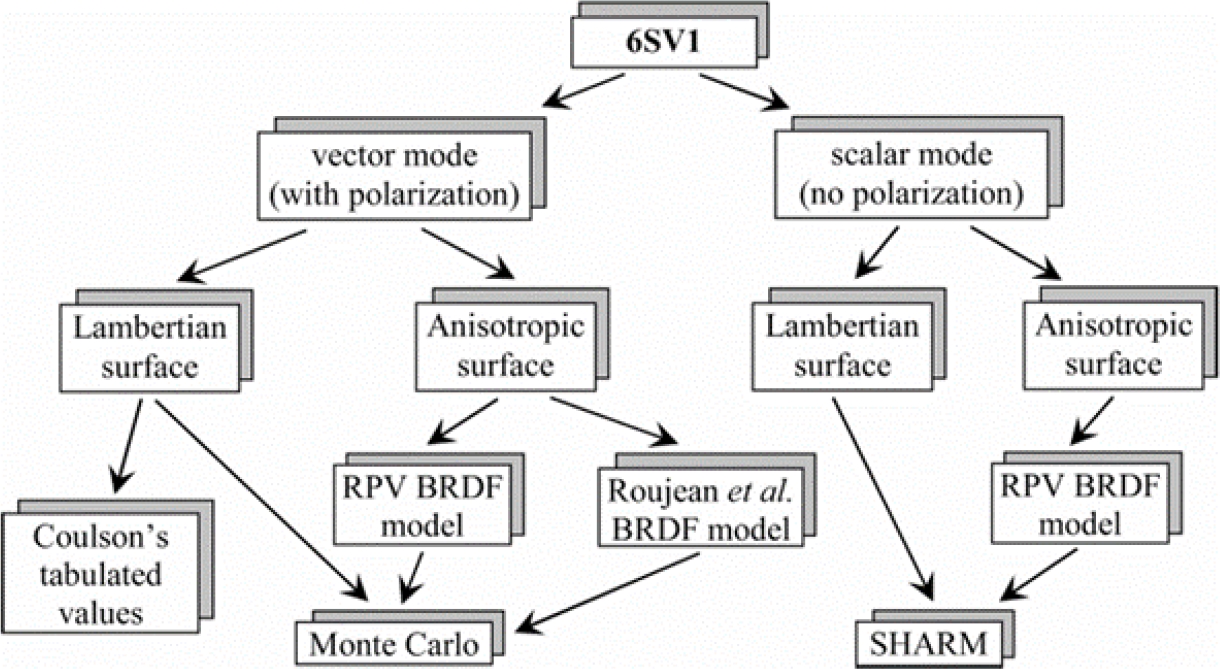
Fig. 1 Flowchart for atmospheric correction of satellite data. Homogeneous Lambertian and anisotropic surfaces. (Adapted from Vermote et al. 2007)
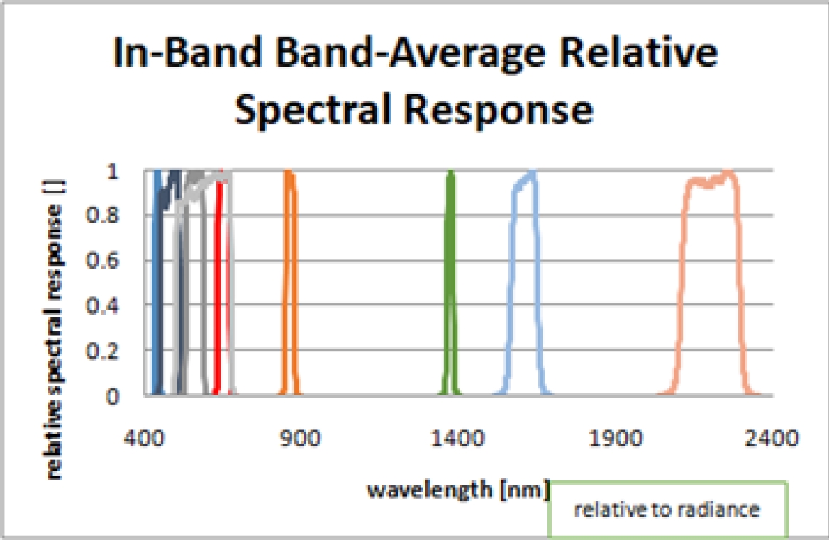
Relative Spectral Response is also used for spectral convolution when doing calibration (i.e. vicarious calibration). The Coastal/Aerosol band was selected randomly, since the objective of this work is to compare the performance of different DL models to emulate the RTC 6S.
As a reference, this band has two cases use, one is to improve the estimation of aerosols to be used in atmospheric correction methods and two, the capture of images of inland waters (i.e. lakes and coasts).
3.2 Atmospheric Correction (AC) in 6S
Radiative Transfer Code 6S allows atmospheric correction of satellite images (i.e. to obtain the reflectance of the Earth's surface). For this, it is necessary to introduce the parameters described above and assume that the surface is isotropic (i.e. Lambertian). Normally the value of the apparent radiance must be entered, that is, the pixel must have previously been converted from its raw value (Digital Number) to radiance. The conversion is done with the following formula [20]:
As with most atmospheric correction algorithms, the correction is done pixel by pixel, except in a few algorithms in which the AC is done band by band as in “Empirical Line Calibration” [6].
3.3 Deep Learning Models Development
Building a robust, accurate, and well-generalized DL model depends on several factors, including preprocessing the training data set, building the network architecture, and finally tuning hyperparameters such as learning rate, the lot size, etc. (Chollet, 2021). The following sections describe these critical factors.
3.3.1 Data Preprocessing
The ranges of all input variables (from uniform distributions) were resized between [0, 1] using Min-Max normalization. In addition, before training the network, the batch data set was shuffled to improve the training convergence and improve the generalization ability of the network [9, 20].
Table 2 Parameters of the MLP
| MLP | Parameters/Hiperparameters | Trainable Parameters |
| Input Variables (Normalized) | SZA, SAA, VAA, AOD, RAD | |
| Activation Function | ReLU (except output layer) | |
| Training Loss Function | MSE | |
| Hidden Layers | 2 | |
| Neurons number in the input layer | 5 | |
| Neurons number in the first hidden layer | 40 | |
| Neurons number in the sencond hidden layer | 60 | |
| Dropout layer | 0.25 (25%) | |
| Neurons number in the output layer | 1, Función de activación: Linear | 60+1=61 |
| Learning rate | 0.001 | |
| Batch Size | 32 | |
| Optimizer | ADAM | |
| Epochs number (Early Stopping) | 50 |
Table 3 Parameters of the 1D-CNN
| 1D-CNN | Inputs/Hiperparameters | Commentary/Train. Param. parameters |
| Input Variables (Normalized) | SZA, SAA, VAA, AOD, RAD | Input as column vector |
| Activation Function | ReLU | Fourth and tenth GeLU |
| Training Loss Function | MSE | Regression |
| Layers Number | 13 | |
| 1st layer: “Reshape” | Target Shape: |
Row vector conversion |
| 2nd layer: “Conv 1D” | Kernels: 32, Size: |
|
| 3rd layer: “Conv 1D” | Kernels: 64, Size: |
|
| 4th layer: “Conv 1D” | Kernels: 128, Size: |
|
| 5th layer: “Conv 1D” | Kernels: 256, Size: |
|
| 6th layer: “Reshape” | Target Shape: |
Row vector conversion |
| 7th layer: “Maxpooling” | Pool size: 2, Strides: 2 | Dimensionality reduction |
| 8th layer: “Flatten” | N/A | MLP input |
| 9th layer: “Dropout” | 0.25 (25%) | Prevent Overfitting |
| 10th layer: “Dense” | 256 neurons | |
| 11th layer: “Dense” | 128 neurons | |
| 12th layer: “Dropout” | 0.25 (25%) | Prevent Overfitting |
| 13th layer: “Densa” | 1 neuron, Activation Function: Linear | |
| Learning rate | 0.001 | |
| Batch Size | 32 | |
| Optimizer | ADAM | |
| Épochs number (Early Stopping) | 8 |
Table 4 Parameters of the MLP + Numerical Embedding
| MLP-NE | Inputs/Hiperparameters | Trainable Parameters |
| Input Variables (Normalized) | SZA, SAA, VAA, AOD, RAD | |
| Activation Function | ReLU (except the “embedding” layer and the output) | |
| Training Loss Function | MSE | |
| Embedding dimensión for each input | 10 (dense layer without activation function) | |
| Number of hidden layers | 2 | |
| Neurons number in the input layer | 50 | |
| Neurons number in the first hidden layer | 40 | |
| Neurons number in the second hidden layer | 60 | |
| Dropout layer | 0.25 (25%) | |
| Neurons number in the output layer | 1, Función de activación: Linear | |
| Learning rate | 0.001 | |
| Batch Size | 32 | |
| Optimizer | ADAM | |
| Epochs number (Early Stopping) | 20 |
3.3.2 Multilayer Perceptron Architecture (MLP)
The model implemented in Keras using the sequential API is as follows.
3.3.3 One Dimension Convolutional Neural Network Architecture (1D-CNN)
The model implemented in Keras using “Functional API” is the following, the model presented in [9] was taken as a base, with some modifications, in particular the input was taken in the form of a vector and no readjustment was made in the form of the input tensor as mentioned in this article. The parameters of the implemented model are the following, the calculation of learning parameters is shown for each layer where there is.
3.3.4 Multilayer Perceptron with Numerical Embedding (MLP-NE)
The model implemented in Keras using “Functional API” is the following.
3.3.5 Vision Transformer Architecture (ViT)
The model implemented in Keras using “Functional API” and “Subclassing” is as follows, each Embedding of each parameter is stacked to form the “array of embeddings”, so that the sequence that is processed is the sequence of parameters. The Vision Transformer architecture was taken as a basis, in which only the encoder is implemented [18, 25].
The dense layers of Query, Key and Value (3 dense layers, see equation), the number of attention heads and the output dense layer are taken into account to reduce the dimension of the concatenation of the attention heads, the formula for calculating the MHSA is then:
All scenarios were implemented on a Windows PC with 3.20 GHz Intel Core i7-8700 CPU and 8 GB RAM. The Adam (Adaptive moment estimation) optimization algorithm was used in all models.
Table 5 Parameters of the ViT
| ViT | Inputs/Hiperparameters | Activation Function | Commentary/Trainable parameters |
| Input Variables (Normalized) | SZA, SAA, VAA, AOD, RAD | N/A | |
| Training Loss Function | MSE | N/A | Regression |
| Embedding dimension for each input variable | Dense layer each parameter without activation function | ||
| Encoders number | 3 | N/A | N/A |
| Attention Heads Number | N/A | N/A | |
| Key Matrix Dimension | N/A | N/A | |
| Encoder | Hiperparameter | Activation Function | Commentary/Trainable parameters |
| 1st Layer: “Normalization” | Epsilon: |
N/A | 64 (obtained from model summary) |
| 2nd layer: “Multi Head Self Attention” | Dropout: 0.1 (10%) | N/A | 8416* (see equation) |
| 3rd layer: “Add” | N/A | N/A | 0 |
| 4th layer: “Normalization” | Epsilon: |
N/A | 64 (obtained from model summary) |
| 5th layer: “Dense” | 64 neurons | GELU (ReLU para el tercer encoder) | |
| 6th layer: “Dense” | 32 neurons | GELU(ReLU para el tercer encoder) | |
| 7th layer: “Dropout” | 0.25 (25%) | N/A | Prevent Overfitting |
| 8th layer: “Add” | N/A | N/A | 0 |
| Output layer | Hiperparameter | Activation Function | Commentary/Trainable parameters |
| 1st layer: “Normalization” | Epsilon: |
N/A | 64 (obtained from model summary) |
| 2nd layer: “Flatten” | N/A | N/A | N/A |
| 3rd layer: “Dense” |
|
ReLU | |
| 4th layer: “Dense” |
|
ReLU | |
| 5th layer: “Dropout” | 0.25(25%) | N/A | N/A |
| 6th layer: “Dense” | 1 neurona | Linear | |
| Total Parameters | |||
| Learning rate | 0.001 | N/A | N/A |
| Batch Size | 32 | ||
| Optimizer | ADAM | ||
| Épochs number (Early Stopping) | 20 | N/A | N/A |
3.4 Performance Evaluation
The performance of the proposed models was evaluated using the test data set. So two criteria were used to make the evaluation before deciding whether to modify the architecture of the models or the hyperparameters, including the root mean square error (RMSE) and the coefficient of determination (R²). For a value of RMSE>0.5 and/or R²<0.6, it was considered that the architecture or hyperparameters should be adjusted iteratively until the acceptable conditions were met. The formulas for these metrics are as follows:
4 Results and Comparison
This section presents the results and the comparison between the different models presented.
4.1 Model Training and Testing in the Simulation Domain
The entire simulated data set (3840 simulations) was divided into two subsets: training and validation, at a proportion respectively of 80% and 20% of the total simulated data set. To ensure an unbiased split of the data set, the data set was used randomly to choose the training and validation data.
Cross-validation of the model was also carried out using the K-Fold method (K=5) [18], that is, the data set was divided into 5 equal parts, so that the validation data set was rotated.
As discussed in the previous section, different scenarios, including varying the network architecture and tuning the network hyperparameters with various values, were evaluated to construct an optimal network for surface reflectance modeling (i.e. atmospheric correction).
As part of these experiments, the following Table provides information on the performance of the models presented above. It is striking that the convolutional model has the worst performance, which may be due to an inadequate number of training data or because it is convenient to use a 3-dimensional input tensor. In fact, in [9] they “reshape” the input vector to convert it into a 3-channel input.
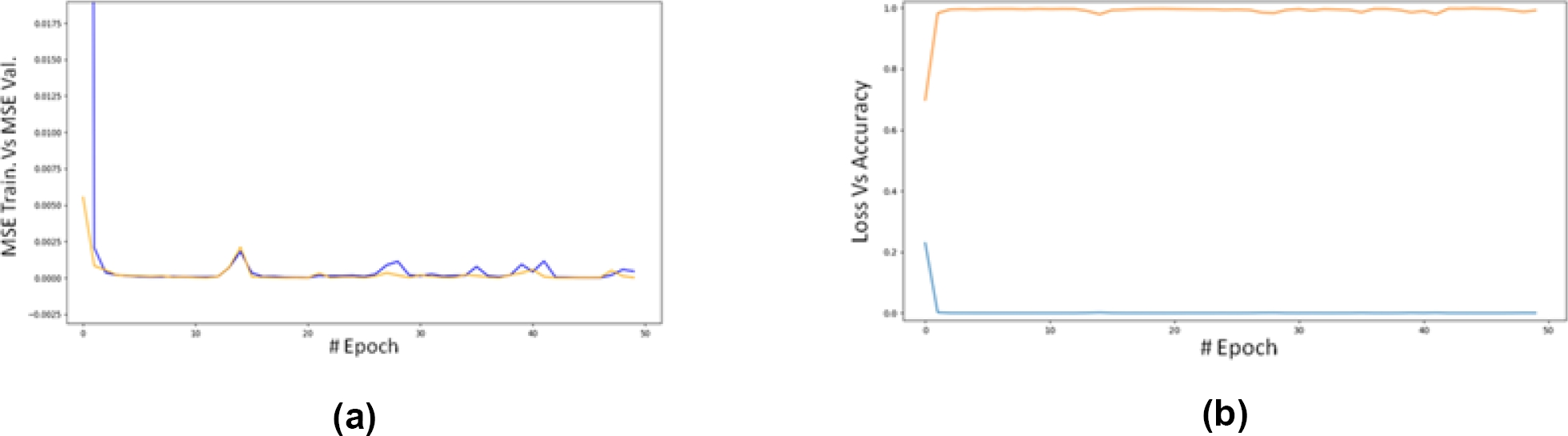
Fig. 5 MSE for training data (blue) and validation data (orange) versus epoch for the 1D-CNN model (a). MSE for training data (blue) and accuracy (R²) for validation data versus epoch for the 1D-CNN model (b)
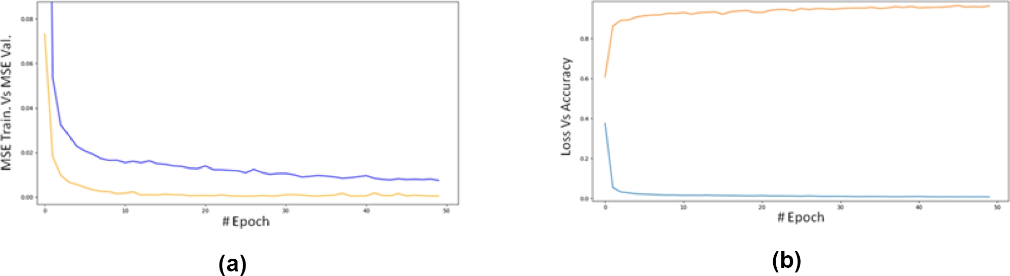
Fig. 6 MSE for training data (blue) and validation data (orange) versus epoch for the MLP model (a). MSE for training data (blue) and accuracy (R²) for validation data versus epoch for the MLP model (b)
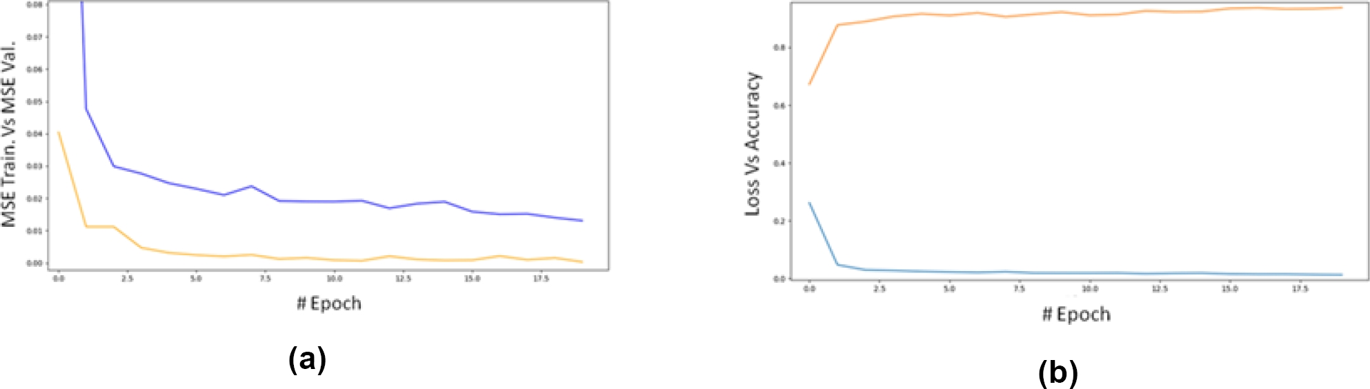
Fig. 7 MSE for training data (blue) and validation data (orange) versus epoch for the MLP-NE model (a). MSE for training data (blue) and accuracy (R²) for validation data versus epoch for the MLP-NE model (b)
For comparison purposes, the results obtained are the following:
An attempt was made to make changes to the architecture of the convolutional model, both by trying to reduce the number of parameters, via reducing the number of filters or kernels, as well as by decreasing the number of layers, however, it was concluded that the problem is the loss of the model's ability to generalize is mainly due to the use of a small data set.
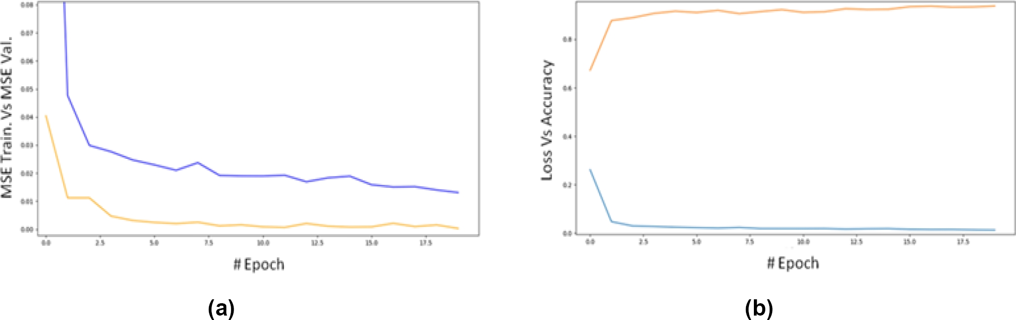
Fig. 8 MSE for training data (blue) and validation data (orange) versus epoch for the ViT model (a). MSE for training data (blue) and accuracy (R²) for validation data versus epoch for the ViT model (b)
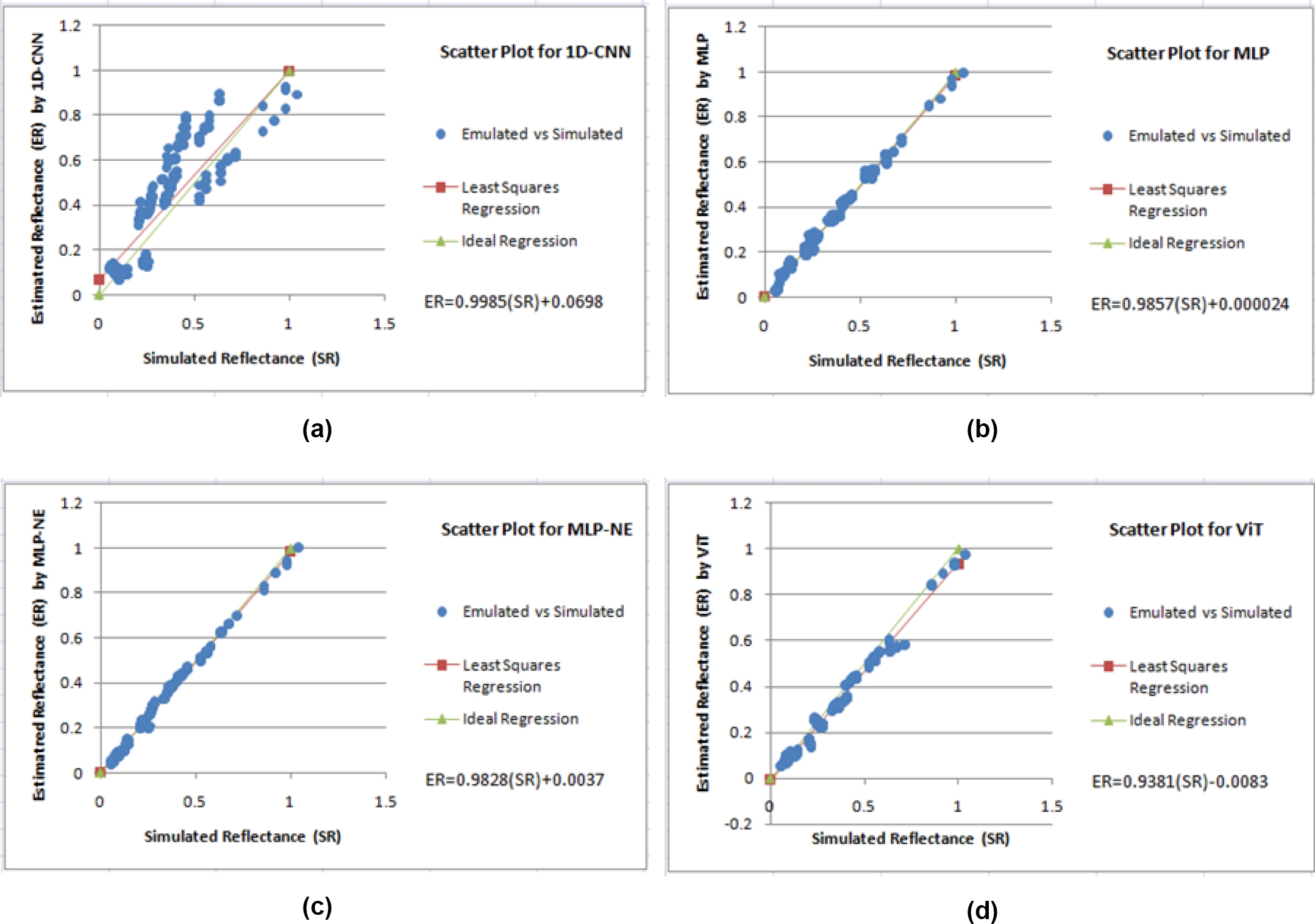
Fig. 9 Dispersion between the simulated reflectance and the reflectance estimated by the 1D-CNN model (a). Dispersion between the simulated reflectance and the reflectance estimated by the MLP model (b). Dispersion between the simulated reflectance and the reflectance estimated by the MLP-NE model (c). Dispersion between the simulated reflectance and the reflectance estimated by the ViT model (d)
Several other attempts were made to improve the generalization ability like layer normalization, but no improvement was observed. As we can see in the previous plots, the MLP-NE model has the best performance of the four evaluated models.
Most of the predicted values of this model do almost a perfect match with the regression line, it is, it shows a strong agreement with the simulated value. Interestingly, the CNN model has the worst performance of all models, the reason behind this behavior could be the small size of the data-set [27].
5 Conclusions
This study presented an emulation-based approach to approximate surface reflectance (Atmospheric Correction) based on RTM using 4 different Deep Learning models. The developed models achieved acceptable precisión and computational speed, except in the convolutional model which, as mentioned above, may be due to insufficient data or the type of vector input.
It could be observed that the convolution model has a notably lower performance than the other models, this is due, as inferred based on the tests carried out, to the fact that the data set is small as explained in [27]. On the other hand, the trained models are applicable only for the defined ranges of inputs in the simulation domain and need retraining in case of changing these ranges for other areas of interest.
The search for a suitable architecture and optimal hyperparameters was based on a trial and error approach, which requires more time and effort to configure. But once the network has been trained and tested, it can operate with acceptable accuracy and speed. More importantly, this effort demonstrated that emulation-based systems using this approach can be an effective solution for establishing the relationship between remote sensing observations and atmospheric and surface parameters.
6 Future Work
Research on this type of models to emulate RTC will be expanded to include at least 100,000 simulations, which according to several authors [9, 22] is enough to adequately train this type of models, so it will possibly be necessary to adjust the model architecture and do new tests. In particular, it is desired to reevaluate the performance of the convolutional model with a larger data set.

