SciELO - Scientific Electronic Library Online

 
vol.28 número4Knowledge Injection for Field of Research Classification and Scholarly Information ProcessingA Study on Content-based Reviewer Assignment in the Semantic Web and Computer Science Domains índice de autoresíndice de materiabúsqueda de artículos
Home Pagelista alfabética de revistas  

Servicios Personalizados

Revista

Articulo

Indicadores

Links relacionados

  • No hay artículos similaresSimilares en SciELO

Compartir


Computación y Sistemas

versión On-line ISSN 2007-9737versión impresa ISSN 1405-5546

Comp. y Sist. vol.28 no.4 Ciudad de México oct./dic. 2024  Epub 25-Mar-2025

https://doi.org/10.13053/cys-28-4-5300 

Articles of the Thematic Section

Branching and Pruning Algorithm for Computing the Merrifield-Simmons Index on Polygonal Grids

Herlinda González-Vázquez1 

Cristina López-Ramírez1  * 

Pedro Bello-López2 

Guillermo de Ita-Luna2 

11 Universidad Juárez Autónoma de Tabasco, División Académica de Ciencias y Tecnologías de la Información, Villahermosa, Mexico. 231H18004@alumno.ujat.mx.

22 Benemérita Universidad Autónoma de Puebla, Facultad de Ciencias de la Computación, Puebla, Mexico. pedro.bello@correo.buap.mx, deitaluna63@gmail.com.


Abstract:

In this paper, we present the molecular structure of benzene as a regular hexagonal ring and an isomorphic hexagonal lattice, a molecular structure introduced by Merrifield-Simmons (MS) in 1989. The MS index, a topological index used in mathematical chemistry, is the number of independent sets of a graph G. This index plays a crucial role in our understanding of complex molecular structures. The strategy to compute the MS index involves the construction of a Hamiltonian trajectory in the input graph. These structures are discussed in fields such as theoretical and computational chemistry. Therefore, we propose a novel branch and bound method for counting independent sets on polygonal benzenoid meshes, highlighting its importance in the study of the analysis of complex molecular structures and its applicability in interdisciplinary scientific fields.

Keywords: Benzenoid; independent sets; Hamiltonian path

1 Introduction

The molecular form of benzene is represented as a regular hexagonal ring, as shown in Figure 1, in which each vertex contains a carbon atom. These carbon atoms are bonded together by alternating single and double bonds.

Fig. 1 Molecular shape of benzene 

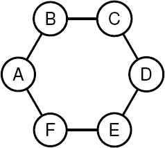
As a result, the benzene molecule is planar and exhibits hexagonal symmetry [6]. An isomorphic hexagonal grid is a grid structure formed by regular hexagons connected to each other.

In a square or rectangular grid, where the grid elements are squares or rectangles, in an isomorphic hexagonal grid, hexagons are the basic units of the grid, forming a polygonal grid, where each polygon shares an edge with the adjacent polygons, which creates a regular and symmetrical structure, as shown in Figure 2.

Fig. 2 Hexagonal mesh 

Therefore, if we consider the molecular structure to be a skeleton, we can represent it as a graph G, where the carbon atoms represent the vertices and the atomic adjacencies are the edges of the graph or edges [9].

The Merrifield-Simmons index (MS) [13], which in graph theory is known as the Fibonacci number of a graph i(G), is a topological index used in mathematical chemistry [7, 15] that represents the number of sets in the graph G.

Independent sets are primarily studied in the field of computer science because graphs are a powerful tool for modeling real-life problems. The aim is to count the independent sets in a set of benzenes that form a polygonal mesh.

Independent sets have potential applications in various areas such as industries, from telecommunications and logistics to finance and strategic planning [16], in addition to improving collaboration and data management. In adiabatic quantum computing, solving the independent set problem involves finding all the computational ground states of a many-body Hamiltonian HG(V,E) [17].

Furthermore, independent sets improve resource allocation and task distribution in computer networks. An exact algorithm, such as branch-and-bound, can solve large networks accurately, as pointed out by [8].

2 Notation

Let G=(V,E) be a simple undirected graph with a set of vertices V and edges E. I(G)= {S/S is an independent set in G}, then I(G) is the set of all independent sets of G. i(G)=|I(G)|, then i(G) is the number of independent sets of G.

The connection between the vertices u and v represent as uv. We also use the notation {u,v} to denote the edge uv. We define N(x)=(yV:{x,y}E) as the neighborhood of xV.

Let’s define some notation. N[x]=N(x){x} represents the closed neighborhood of x. We use |A| to denote the cardinality of a set A. Similarly, the degree of a vertex x is denoted as δ(x)=|N(x)|, while the degree of the graph G is Δ(G)=max{δ(x):xV}.

A set SV(G) of vertices of G is an independent set in G if, for any pair of vertices (u,v)S, then (u,v) are not adjacent in G. Let vV(G). Iv(G)={SI(G):vS}, Iv(G)={SI(G):vS}.

For the computation of the MS index, different algorithms have been developed for counting independent sets in flat grid structures that facilitate counting by applying the traversal by rows and columns or vice versa [3]. In our practical proposal, the main element is to assign a charge (αv,βv) to each vertex v of the graph.

This charge (αv,βv) will be computed while visiting v during a traversal of G, ensuring a straightforward and efficient process.

(αv,βv)=(|Iv(G)|,|Iv(G)|) denotes the vertex charge vV(G). To process the number of independent sets on any path Pn, we will use a computing thread or simply a thread.

A compute thread is a sequence of pairs (αvi,βvi), i=1,,n, which is used during the incremental calculation of i(Pn), i=1,,n, where the n edges of Pn are tree edges, and each pair (αvi,βvi) indicates the charge for vertex vi.

We symbolize with when the Fibonacci rule is applied. In the Hamiltonian path in a graph, we symbolize the start of the walk with |-, and the end with >|. In the mathematical field of graph theory, a Hamiltonian path is defined as a sequence of consecutive edges in a graph where all vertices are visited exactly once. If the last vertex visited is adjacent to the first, it is called a Hamiltonian cycle.

3 Polygonal Topology for Counting Independent Sets

We propose creating an innovative algorithm designed to compute the Merrifield–Simmons index in regular benzenoid systems Hr,t, which consist of hexagonal grids with r rows and t columns, as shown in Figure 3. This algorithm starts with a linear-time Hamiltonian walk on an isomorphic hexagonal grid of Hr,t, while simultaneously incrementally computing the number of independent sets. The time complexity of this approach is lower than that of the transfer matrix method when applied to the calculation of the MS index on grid graphs [5].

Fig. 3 A benzenoid system Hr,t 

3.1 Strategies for Calculating the Merrifield–Simmons Index

3.1.1 Depth First Search

DFS, or depth-first search algorithm, is recognized for providing the steps to explore all the graph nodes without repeating any of them. Figure 4 shows the path DFS(G,v) in depth with the origin node A. The idea is:

  • – The node v is marked.

  • – If all nodes adjacent to v are marked, then TERMINATE; otherwise, a node w adjacent to v that is not marked is chosen.

  • – The process DFS(G,w) is executed.

Fig. 4 DFS route (A, B, E, F, C, G, I, J, H, D) 

3.1.2 Hamiltonian Path

The first step of our method for counting independent sets in a graph involves the construction of a Hamiltonian path (Hc) over the input graph G. During this traversal, Hc visits each vertex of the graph exactly once, identifying each edge of the graph as a tree edge or a frond edge.

Although finding a Hamiltonian cycle in any graph is a classic NP-Complete problem, in this case, the constraints are relaxed by considering paths instead of cycles, which avoids returning to the same starting point.

This relaxation is most evident when examining graph topologies such as meshes, where the searching for an Hc becomes a linear time complexity problem. An example is the case of regular meshes, where Hc can follow a route through rows, alternating directions in odd and even rows.

3.1.3 Fibonacci Calculation in Graphs

Counting the number of independent sets i(G) in a graph G involves traversing the Hamiltonian path Hc of G [4]. During this traversal, the first pair of values starts with (αi,βi)=(1,1). For the following identified edges, one of two rules applies. The Fibonacci recurrence rule:

  1. When the visited edge is a tree edge or a subtraction rule,

  2. When a frond edge is recognized (or back edge if referring to depth-first searches).

If we consider that vi belongs to the path Pn, and vi+1 is the next vertex that will visit an edge of the tree (vi,vi+1), then the following recurrence equation is applied to compute the charge (αvi+1,βvi+1) as a function of the charge (αvi,βvi):

(αvi+1,βvi+1):αvi+1=αvi+βvi, (1)

βvi+1=αvi. (2)

We call the previous pair of recurrences the Fibonacci rule recurrence because when they are applied to a path Pnth, we obtain the knowledge identity i(Pn)=αvi+1+βvi+1=Fn+Fn+1=Fn+2, where Fn is the n-th Fibonacci number:

(αw,βw)i=(αw,βw)(0,βvw)=(αw,βwβv,w). (3)

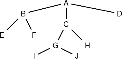
Let us illustrate our proposal with an example; in Figure 5, we show how to compute the MS index of the graph. The Hamiltonian path used to traverse G is ABCDE. A primary thread Lp is opened, and the recurrence function (1) is applied at the beginning of the computation of i(G5):Lp:(1,1)(2,1)(3,2)(5,3)(8,5). Note that temporary charges (αvi,βvi) can be stored in the vertex vi and marked as visited. For any pair of vertices (v,w)S, where S is an independent set and v, w are adjacent, and if edge (v,w) is identified as a frond edge, in this case (E,B) is the frond edge, a secondary thread Ls parallel to Lp is opened; that is, Ls:(0,1)(1,0)(1,1)(2,1) when the walk visits vertex v and w have already been visited, then the subtraction rule (2) is applied, which allows the computation of the charge of vertex v based on a charge of vertex u; and for each frond edge that is encountered. Section 3.2.5 explains this in detail. Therefore:

i(G)=|{0},{A},{B},{C},{D},{E},{A,C},{B,D},{C,E},{E,A},{D,A},{A,C,E}}|=12. (4)

SV(G) is an independent set. If Δx, yS, {x,y}E. i(G)=S/S.

Fig. 5 Graph G with 5 vertices 

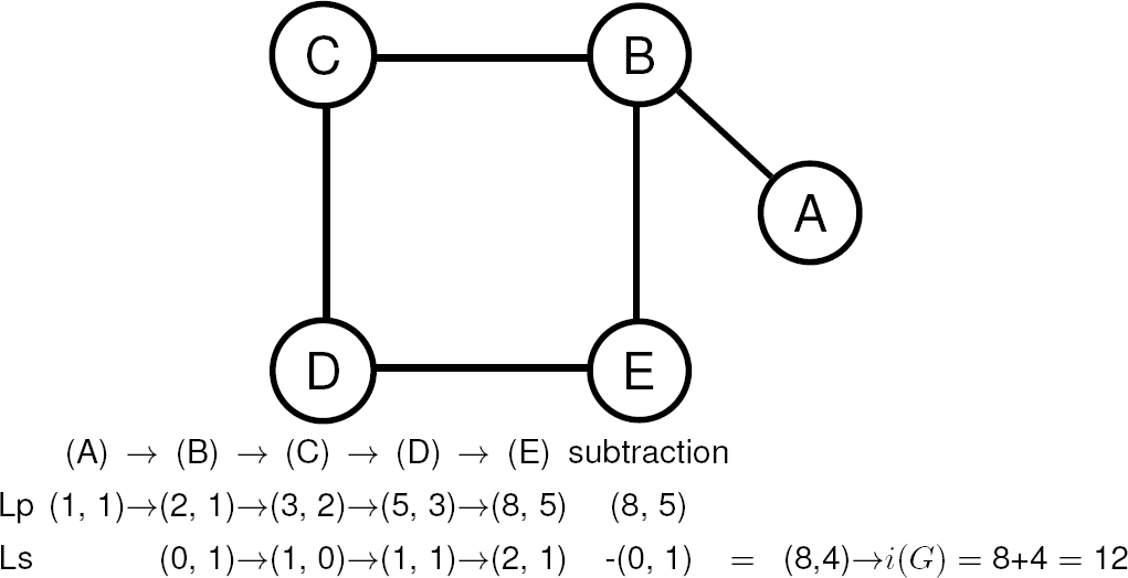
Continuing with our systematic approach, the binary tree in Figure 6 presents all possible combinations formed with the five vertices of graph G, considering that none of its vertices is adjacent to another [1]. The negative symbol indicates that the vertex cannot be part of the combination.

Fig. 6 Binary tree of independent sets. Eliminate vertices B and E, which are frond edges 

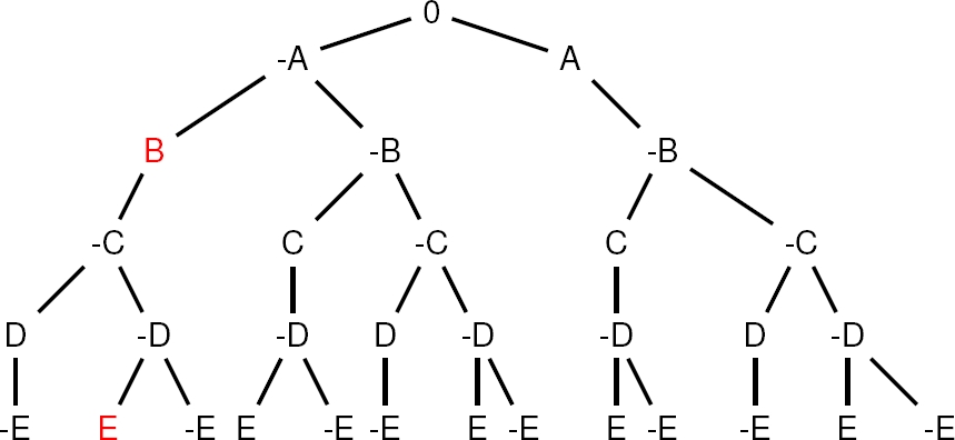
At the end of the construction of the binary tree, we can see that there are 12 independent sets (and we eliminate vertices B and E, which form the frond edge). Moreover, applying the Fibonacci sequence count from Table 1, we confirm that the results, which are of significant importance, coincide.

Table 1 Counting independent sets by the Fibonacci sequence 

Thread A B C D E i(G)
(α1,β1) (α2,β2) (α3,β3) (α4,β4) (α5,β5)
Lp (1,1) (2,1) (3,2) (5,3) (8,5) (8,5)
Ls (0,1) (1,0) (1,1) (2,1) (0,1) (8,4)i(G)=8+4=12

3.2 Counting Independent Sets in Basic Topologies

3.2.1 Linear Chain Graph

Let G=(V,E) with Δ(G)=2 being G a chain graph with n nodes, therefore |V|=n and |E|=m=n1.

Let us order the nodes in G as V={v1,v2,,vn} in such a way that it is fulfilled E={c1,,cn1}={{v1,v2},{v2,v3},,{vn2,vn1},{vn1,vn}}, i.e. |v(ci)v(ci+1)|=1, i=1,,n2. Gi, i={1,,n} being Gi the induced subgraph of G.

The basic technique for counting the number of independent sets i(Gi) on Gi of G is an incremental strategy [12, 11] that is based on associating a pair of values (αi,βi) to each node viV, i={1,,n}.

The path starts at one of the ends of the node v1 or the node vn, visiting its adjacent node linearly. The first pair of values starts with (αi,βi)=(1,1).

The recurrence relation considers that the value is known (αi,βi) associated with the induced subgraph Gi of G such that i(Gi)=(αi,βi).

The new pair of values (αi+1,βi+1) is constructed based on (αi,βi) applying the recurrence it generates to the Fibonacci numbers αi+1=αi+βi, βi+1=αi.

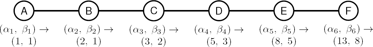
Table 2 shows the counting of independent sets obtained by applying the Fibonacci sequence in the chain graph shown in Figure 7. Therefore, (αi,βi)=(Fi+1,Fi) then i(Gi)=αi+βi=Fi+1+Fi=Fi+2, i={0,,n}, i.e., for n=6, i(G)=i(G6)=F7+F6=F8=21.

Table 2 Independent sets of the linear chain graph 

A B C D E F
(α1,β1) (α2,β2) (α3,β3) (α4,β4) (α5,β5) (α6,β6)
(1,1) (2,1) (3,2) (5,3) (8,5) (13,8)
(F2,F1) (F3,F2) (F4,F3) (F5,F4) (F6,F5) (F7,F6)a

Fig. 7 Linear chain 

3.2.2 Simple Cycle of a Graph

Figure 8 shows a graph containing a simple cycle. Counting independent sets starts a main thread
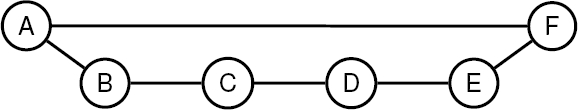
 (Lp); the value pair starts with (αi,βi)=(1,1), and the secondary thread (Ls) starts the sequence recurrence with (αi,βi)=(0,1), where i=1,,m.

Fig. 8 Simple cycle 

The last pair is (αm,βm)=(0,βm) so that the series ((α1,β1)=(0,1)(α2,β2)=(1,0)(α3,β3)=(1,1)(αm,βm)(0,βm)) gives us the value of |Si(G):v1SvmS|. The above series corresponds to the following series considering the Fibonacci numbers:

F0=0 and F1=1, (F0,F1)(F1,F0)(F2,F1)(Fm1,Fm2). (αm,βm)=(0,βm); i(Gc)=((αm,βm)(0,βαm)).

For computing the closing of the cycle [2], we apply rule (2); the last pair (αm,βm) of the secondary thread (Ls) is (αm,βm)=(0,βm), where {vm,v0}E(G) represents the backward edge that closes the cycle of G and is subtracted from the last pair of the primary thread (Lp).

Therefore, ((αm,βm)(0,βm))=((α6,β6)(0,β6))=(13,8)(0,3)=(13,5), we obtain that i(Gc)=13+5, i. e., 18 is the total number of independent sets. This count is shown in detail in Table 3, where we can see the counting of independent sets of G.

Table 3 Independent sets of simple cycle graphs 

Hilo A B C D E F
(α1,β1) (α2,β2) (α3,β3) (α4,β4) (α5,β5) (α6,β6)
Lp (1,1) (2,1) (3,2) (5,3) (8,5) (13,8) (13,8)*
Ls (0,1) (1,0) (1,1) (2,1) (3,2) (5,3) (0,3)**
F0=0,F1=1 (F2,F1) (F3,F2) (F4,F3) (F5,F4) (F6,F5) (F7,F6) (13,5)

*The final pair of the graph cycle αm and βm

**Subtracted rule applied to the edge {F,A}{F , A}.

3.2.3 Cycle and Linear Chain of a Graph

Figure 9 shows a graph with nine nodes, where the nodes A, B, C, D, E, F, and A form a cycle. The exact process is followed to count the independent sets in a cycle for a simple cycle graph, previously studied in Section 3.2.2; the computation is shown in detail in Table 4.

Fig. 9 Simple cycle and linear chain 

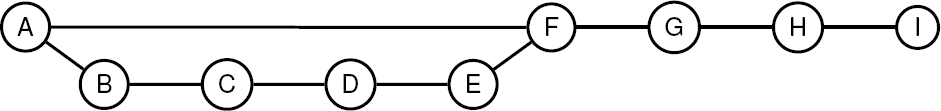
Table 4 Independent sets of the graph simple cycle and linear chain 

Hilo A B C D E F G H I
“ ” (α1,β1) (α2,β2) (α3,β3) (α4,β4) (α5,β5) (α6,β6) (α7,β7) (α8,β8) (α9,β9)
Lp (1,1) (2,1) (3,2) (5,3) (8,5) (13,8)
Ls (0,1) (1,0) (1,1) (2,1) (3,2) (5,3)
(13,5) (18,13) (31,18) (49,31)*

*End Counting Pair (αm,βm)

When node F closes the cycle, the inverse edge rule (2) is applied, obtaining as a result the pair (13,5) and continuing with the computing of the linear sequence applying the Fibonacci rule (1) on the nodes G, H, I until finishing the path of the graph. The total number of independent sets i(G) equals the sum of the last pair (49,31)=49+31, i. e., 80 independent sets.

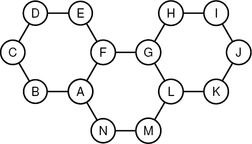
3.2.4 Hexagons Connected by Edges

Figure 10 shows the case of a graph with two cycles connected by a bridge edge. Here, the same process is performed for the simple cycles, and once a back edge is found, the first cycle is closed, equation
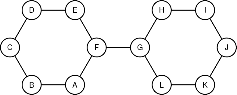
 (2) is applied, and we continue to compute the independent sets according to the Fibonacci rule. Tables 5 and 6 show that the calculations of the total of the independent sets i(G) that it is equal to the sum of the last pair (209,90)=209+90=299 independent sets.

Fig. 10 Two hexagons joined by an edge 

Table 5 Cycle 1 

Hilo A B C D E F
(α1,β1) (α2,β2) (α3,β3) (α4,β4) (α5,β5) (α6,β6)
Lp (1,1) (2,1) (3,2) (5,3) (8,5) (13,8) (13,8)
Ls (0,1) (1,0) (1,1) (2,1) (3,2) (5,3) (0,3)*
(13,5)**

*Applying subtracted rule to the frond edge {F,A}

**Cycle 1 closing pair

Table 6 Cycle 2 

Hilo G H I J K L
(α1,β1) (α2,β2) (α3,β3) (α4,β4) (α5,β5) (α6,β6)
Lp (18,13) (31,18) (49,31) (80,49) (129,80) (209,129)
Ls (0,13) (13,0) (13,13) (26,13) (39,26) (65,39)
(209,129)
(0,39)*
(209,90)

*Applying subtracted rule to the frond edge {L,G}.

3.2.5 Hexagons Connected by Vertices

Algorithms have been developed for counting independent sets in flat grid structures that facilitate counting, applying the traversal by rows and columns or vice versa [3]. Our algorithmic proposal processes the frond edges in two phases. Let v, w be a frond edge of a graph G.

In the first phase, when a walk (Lp) main thread visits the first vertex v of the front edge, the number of active threads and computing threads (Ls) must be duplicated. Assume (αv,βv)i is the charge associated with the active thread Li when visiting vertex v. A new thread Lvwi is created, which is subordinate to the master thread Li, and with an associated initial pair (0,βv)vw.

Therefore, the label vwi of Lvwi is also a pointer to its master thread Li. The second phase in the frond edge processing (v,w) is when the walk visits vertex w, and v has already been labeled as a visited vertex. Thus, control is maintained at vertex w. Suppose (αw,βw)i is the charge of vertex w on the master thread Li.

Meanwhile, (αvw,βvw)vw is the charge of w on the subordinate thread Lvwi. Then, the subtraction rule of equation (2) updates the charge of w in Li. After the application of this rule, the subordinate thread Lvwi is closed. In this way, any thread where the particle vw appears must be closed, which decreases the number of active threads.

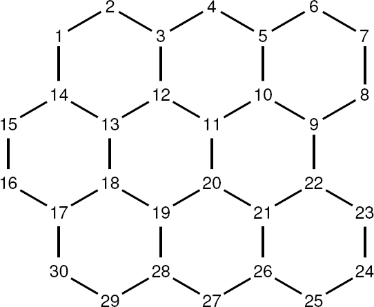
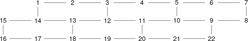
To compute the number of independent sets of a grid is possible by taking the Hamiltonian path Hc as a guide, although the time complexity is of exponential order over the maximum number of frond edges in any row of the grid, given the number of cycles that are kept open during the Hc path. The Fibonacci and subtraction rules are sufficient to process one row of tiles from a hexagonal grid, as shown in Figures 11, 12 and Table 7.

Fig. 11 Three hexagons connected by vertices 

Fig. 12 Grid of three hexagons connected by vertices 

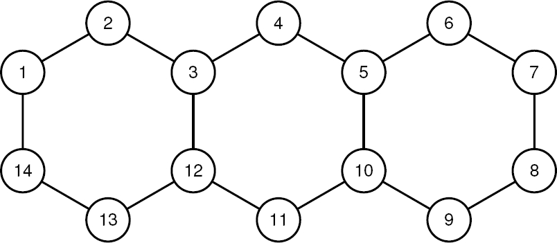
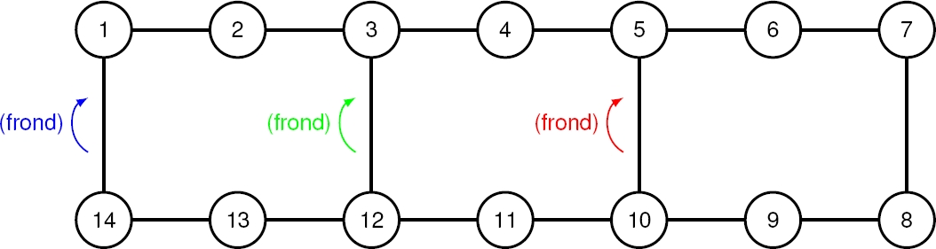
Table 7 Counting of independent sets of Fig. 12 

Element 1 Element 2 Element 3
1 2 3 4 5 6 7 8 9 10 11 12 13 14
Lp(1,1) (2,1) (3,2) (5,3) (8,5) (13,8) (21,13) (34,21) (55,34) (89,55) (0,15)= (89,40)
Ls(0,1) (1,0) (1,1) (2,1) (3,2) (5,3) (8,5) (13,8) (21,13) (34,21) (0,6)= (34,15)
c2Lp (0,2) (2,0) (2,2) (4,2) (6,4) (10,6) (16,10) (26,16) (0,6)= (26,10)
c2Ls (0,1) (1,0) (1,1) (2,1) (3,2) (5,3) (8,5) (13,8) (0,3)= (13,5)
c3Lp (0,5) (5,0) (5,5) (10,5) (15,10) (25,15) ×
c3Ls (0,2) (2,0) (2,2) (4,2) (6,4) (10,6) ×
c2c2Lp (0,2) (2,0) (2,2) (4,2) (6,4) (10,6) ×
c3c2Lp (0,1) (1,0) (1,1) (2,1) (3,2) (5,3) ×
(129,89) (218,129) (311,218) (529,311)
(0,36) (0,114)
=(218,93) =(529,197)
(49,34) (83,49) (114,83) (197,114)
(0,18) ×
=(83,31)
(36,10) (46,36) ×
(18,13) =(31,18) ×

4 A Branch-and-bound Algorithm

4.1 Benzenoid System

The first stage in our method for computing the Merrifield-Simmons index in benzenoids I(Hr,t) involves inserting the benzenoid system Hr,t from Figure 3 into a regular hexagonal grid HG resulting as in Figure 13, where instead of conventional squares, we consider hexagons.

Fig. 13 Regular hexagonal mesh HGm,n 

Both graphs, the benzenoid system Hr,t and the regular hexagonal grid HG, are isomorphic and possess the same number of hexagons. We designate the number of rows in HG as m and the number of columns in the first row as n.

Therefore, HGm,n represents a hexagonal mesh with m rows, where each row has n or n+1 columns. The first row in HGm,n has n vertices, while rows 2 and 3 have n+1 vertices. Row 4 again has n vertices, and the next two rows have n+1 vertices, and so on. The number of hexagons is the same in each row of HGm,n, so the hexagons in Hr,t are one-to-one related to the hexagons in HGm,n.

The insertion of a benzenoid system Hr,t into a regular hexagonal grid HGm,n can be performed in linear time in rt, thanks to the existence of linear time algorithms that create insertion of a planar graph into a grid [14]. Therefore, we can represent the edges of HGm,n as straight line segments. HGm,n has only vertices of degree two or three.

The edges are divided into two types: Horizontal edges with vertices {(i,j),(i,j+1)}, where i=1,,m y j=1,,n; and vertical edges with vertices {(i,j),(i+1,j)} or {(i,j),(i+1,j+1)}, or {(i,j),(i+1,j1)} depending on the row under consideration.

4.2 Branch and Pruning

  1. Hamiltonian Path: The Hamiltonian path It can be formed based on a path through grid rows by changing the path direction from left to right over odd rows, and with a path from right to left for even rows. We start with constructing a Hamiltonian path Iv(G) that traverses each vertex of HGm,n once.

    1. For vertices of degree 2, δ(v)=2 the walker visits both edges and continues the path; for vertices of degree 3, δ(v)=3 the walker visits all three edges and checks whether the degree of its neighbors equals three. If δ(N(v))=3, N(v)=3, then v is the vertex selected to apply pruning, as shown in Figure 14 subsection (a).

  2. Counting Rules: Set of counting rules to be applied to the edges (or vertices) during the path [10]:

    • (a) Branching rule:

i(G)=i(Gv)+i(GN[v]). (5)

  1.  

    • (b) The vertex to be selected must be of degree 3, that is, δ(v)=3; for example, in Figure 14 section (a), the vertex that has been selected is shown.

    • (c) Its neighbors must also be of degree 3, that is, δ(N(v))=3; in Figure 14 part (b), you can see which are the neighbors of v, in this case, they are {12,10,20}.

Fig. 14 Branching and pruning 

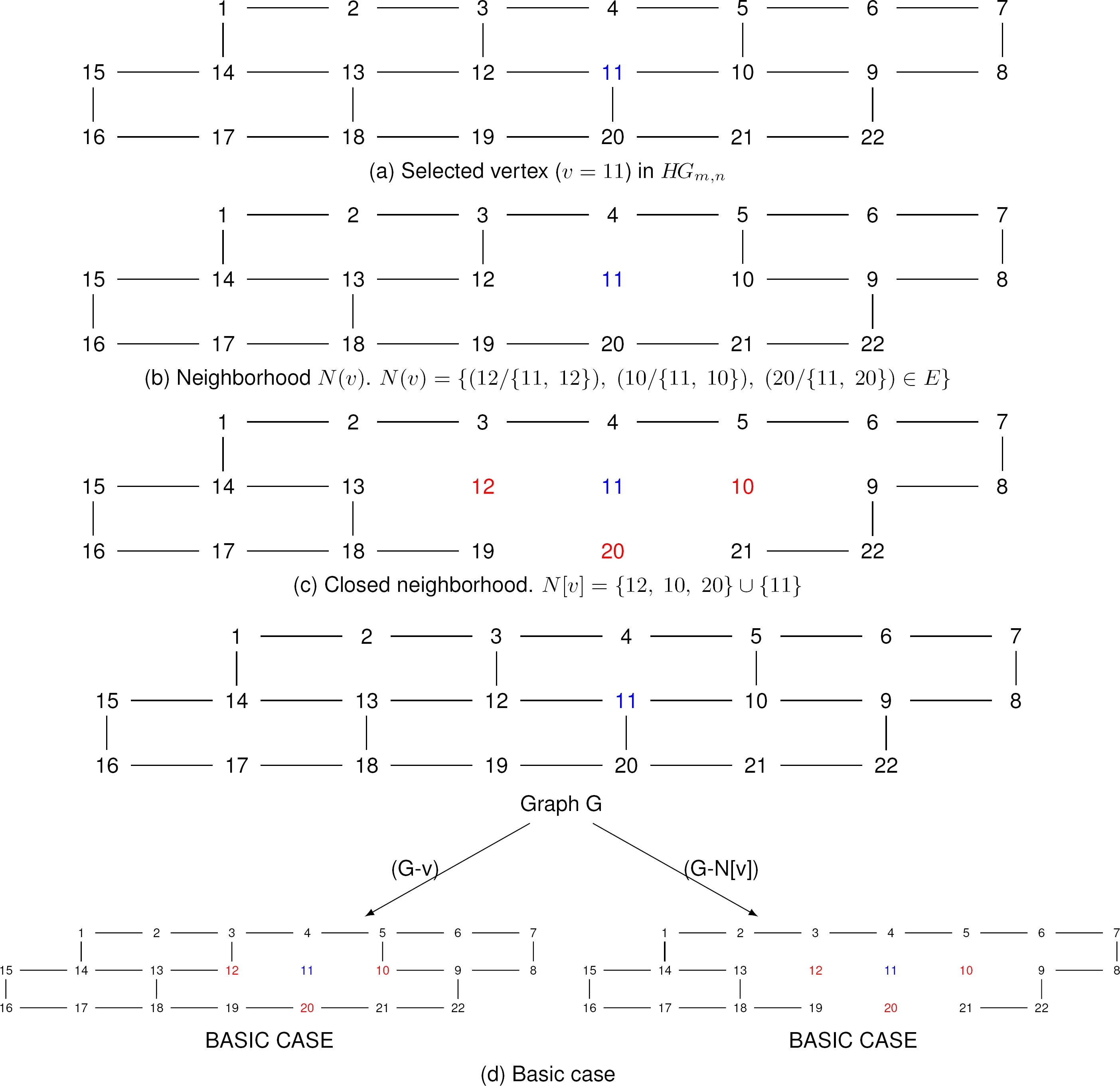
Implementing the branching rule (3) at vertex v generates two nodes, v1 and v2, from the current node in the calculation tree. The subgraph associated with v1 is established as: G1=(Gv), while the subgraph associated with v2 is established as G2=(GN[v]). We have a similar problem for each subgraph Gi, i=1,2 that we had with the original grid HG.

If we solve the problem recursively and ri is its solution, then the complete solution for r=i(HG) is r=r1+r2. The previous procedure determines an enumerative tree whose leaves correspond to the instances of subgraphs called the basic cases of the enumerative tree.

The branching process is iterated until the path of the entire graph is complete and the Hamiltonian path walker does not find another vertex that satisfies the rules. It is time to apply the independent set counting to the resulting basic cases, shown in Figure 14 subsection (d), using the Fibonacci series.

Once we have defined the basic cases, we apply the computational strategies for counting independent sets in simple basic structures and mesh structures, such as linear chain, simple cycle, simple cycle and linear chain, hexagons connected by edges, and hexagons connected by vertices, as it was presented in Section 3.2.

The time complexity of the branch-and-prune algorithm is determined by the recurrence I(G)=i(Gv)+i(GN[v]). Our proposal still exhibits exponential time complexity but does not exhibit the explosive combinatorial character that the classical transfer matrix method has for computing i(HGm,n).

5 Conclusion and Future Work

We have presented a branching-and-pruning proposal for computing the number of independent sets in hexagonal meshes, denoted as HGm,n, where m represents the number of rows and n the number of columns. In our approach, we use the branching rule to split the graph into simpler subgraphs. Our strategy consists of decomposing the original graph into outer flat subgraphs, treating them as basic cases. The time complexity of our approach to this computation is significantly lower than that required by the classical transfer matrix method to achieve the same result.

In the future we plan to investigate combinatorial optimization techniques to reduce the complexity of the branching-and-pruning algorithm for computing independent sets on hexagonal meshes, and further improve our understanding and ability to address this computational challenge more effectively. This will allow us to deal more efficiently with larger graphs. Thus, this proposal could be applied as an effective solution for processing BIG DATA and other complex networks by optimizing node selection and network reduction.

Acknowledgments

The authors give thanks to Conahcyt-México for the economical support for this researching.

References

1. Bracho, R. L., Sánchez, M. P. O. (2000). Un algoritmo paralelo para el problema del conjunto independiente. Revista de Matemática: Teoría y Aplicaciones, Vol. 7, No. 1–2, pp. 125–134. DOI: 10.15517/rmta.v7i1-2.185. [ Links ]

2. de-Ita, G., Rodríguez, M., Bello, P., Contreras, M. (2020). Basic pattern graphs for the efficient computation of its number of independent sets. Pattern Recognition, Vol. 12088, pp. 57–66. DOI: 10.1007/978-3-030-49076-86. [ Links ]

3. de-Ita-Luna, G., Vidal, M. T., Loranca, B. B. (2023). A novel method for counting independent sets in a grid graph. International Journal of Combinatorial Optimization Problems and Informatics, Vol. 14, No. 1. [ Links ]

4. El-Basil, S. (1988). Theory and computational applications of Fibonacci graphs. Journal of Mathematical Chemistry, Vol. 2, No. 1, pp. 1–29. DOI: 10.1007/BF01166466. [ Links ]

5. Euler, R. (2005). The Fibonacci number of a grid graph and a new class of integer sequences. Journal of Integer Sequences, Vol. 8, No. 2. [ Links ]

6. Gutman, I. (1982). Topological properties of benzenoid systems IX on the sextet polynomial. Zeitschrift für Naturforschung A, Vol. 37, No. 1, pp. 69–73. DOI: 10.1515/zna-1982-0115. [ Links ]

7. Hosoya, H. (1973). Topological index and Fibonacci numbers with relation to chemistry. Fibonacci Quart, Vol. 11, No. 3, pp. 255–266. DOI: 10.1080/00150517.1973.12430822. [ Links ]

8. Lamm, S., Sanders, P., Schulz, C., Strash, D., Werneck, R. F. (2015). Finding near-optimal independent sets at scale. Proceedings of the Eighteenth Workshop on Algorithm Engineering and Experiments, pp. 138–150. DOI: 10.1137/1.9781611974317.12. [ Links ]

9. Merrifield, R. E., Simmons, H. E. (1980). The structures of molecular topological spaces. Theoretica chimica acta, Vol. 55, No. 1, pp. 55–75. DOI: 10.1007/BF00551410. [ Links ]

10. Morrison, D. R., Jacobson, S. H., Sauppe, J. J., Sewell, E. C. (2016). Branch-and-bound algorithms: A survey of recent advances in searching, branching, and pruning. Discrete Optimization, Vol. 19, pp. 79–102. DOI: 10.1016/j.disopt.2016.01.005. [ Links ]

11. Okamoto, Y., Uno, T., Uehara, R. (2005). Linear-time counting algorithms for independent sets in chordal graphs. pp. 433–444. DOI: 10.1007/11604686_38. [ Links ]

12. Samotij, W. (2015). Counting independent sets in graphs. European Journal of Combinatorics, Vol. 48, pp. 5–18. DOI: 10.1016/j.ejc.2015.02.005. [ Links ]

13. Simmons, H. E., Merrifield, R. E. (1977). Mathematical description of molecular structure: Molecular topology. Proceedings of the National Academy of Sciences, Vol. 74, No. 7, pp. 2616–2619. DOI: 10.1073/pnas.74.7.2616. [ Links ]

14. Vadhan, S. P. (2001). The complexity of counting in sparse, regular, and planar graphs. SIAM Journal on Computing, Vol. 31, No. 2, pp. 398–427. DOI: 10.1137/S0097539797321602. [ Links ]

15. Vesel, A. (2013). Fibonacci dimension of the resonance graphs of catacondensed benzenoid graphs. Discrete Applied Mathematics, Vol. 161, No. 13, pp. 2158–2168. DOI: 10.1016/j.dam.2013.03.019. [ Links ]

16. Wurtz, J., Lopes, P. L. S., Gorgulla, C., Gemelke, N., Keesling, A., Wang, S. (2022). Industry applications of neutral-atom quantum computing solving independent set problems. DOI: 10.48550/ARXIV.2205.08500. [ Links ]

17. Yin, X. F., Yao, X. C., Wu, B., Fei, Y. Y., Mao, Y., Zhang, R., Liu, L. Z., Wang, Z., Li, L., Liu, N. L., Wilczek, F., Chen, Y. A., Pan, J. W. (2023). Solving independent set problems with photonic quantum circuits. Proceedings of the National Academy of Sciences, Vol. 120, No. 22. DOI: 10.1073/pnas.2212323120. [ Links ]

Received: April 14, 2024; Accepted: July 07, 2024

* Corresponding author: Cristina López-Ramírez, e-mail: cristina.lopez@ujat.mx

Creative Commons License This is an open-access article distributed under the terms of the Creative Commons Attribution License