


 nueva página del texto (beta)
 Inglés (pdf)
 Artículo en XML
 Referencias del artículo
 Enviar artículo por email
 Citado por SciELO
  Similares en
SciELO
Similares en
SciELO 
 Permalink
1 Introduction
According to the World Health Organization (WHO) [29], falls constitute the second leading cause of unintentional injury death worldwide.
Each year, 37.3 million falls require medical attention, and an estimated 684,000 become fatal. Notably, adults older than 60 years suffer the most significant number of fatal falls or serious injuries. Almost 30% of adults over 65 years report at least one fall yearly [1], increasing the risk with age [29].
The most common causes of falls in elderly individuals are environment-related factors and disorders related to gait, balance, or weakness [24]. Additionally, older individuals with mobility impairments, cognitive deficits, chronic conditions, geriatric syndromes, and the use of particular medications are at an increased risk of experiencing falls [12].
From a financial perspective, elderly falls impact the economic concerns of government-funded programs. Several studies estimated annual costs of billions of dollars in expenditures for medical fall treatments [6]. Moreover, the economic burden would be expected to grow due to the rising life expectancy, leading to a larger aging population.
As reported by the WHO, the population of individuals older than 60 will double (2.1 billion) by 2050, which is 22% of the global population [28]. Therefore, identifying strategies for fall prevention and early detection in elderly individuals becomes a topic of relevance. Over the past decades, fall prevention and detection have been active research areas [23]. Several strategies, including risk factors reduction, exercise routines, environmental modifications, and education programs, have demonstrated effectiveness in preventing falls [24]. However, while fall prevention can reduce the occurrence of falls, it does not eliminate the possibility of a fall event.
Conversely, fall detection techniques focus on recognizing falls and alerting when a fall event has occurred [27]. In this work, we introduced a fall detection model based on non-wearable devices and machine learning techniques.
The main contributions of this study are, firstly, the establishment of a dataset containing room temperature values through the utilization of a thermal sensor and, secondly, the application of machine learning techniques for the classification of fall and non-fall events.
2 Related Work
Fall detector methods can be broadly categorized into wearable and non-wearable device-based approaches. Wearable devices rely on clothing embedded with sensors, including accelerometers, gyroscopes, electro-myography, and pressure sensors, to discern the subject’s motion and location [19, 23].
Accelerometers, in particular, have been widely used for fall detection in wearable systems [19]. However, wearable-based systems may not be a good choice for older adults. Wearable devices require subjects to wear the sensors actively and, in some cases, need to be constantly charging (e.g., smartwatches, smartphones).
Moreover, wearable devices may be uncomfortable, easily misplaced, or forgotten by elderly individuals. Unlike wearable devices, non-wearable devices are less invasive. Non-wearable devices can be further divided into ambiance and vision-based sensors.
Sound, temperature, visual, and vibrational sensors, among others, fall into the category of non-wearable devices [19, 23]. Díaz-Ramírez et al. [5] introduced a wireless sensor network (WSN)-based fall detection system that relies on sound analysis. In this system, nodes detect falls by analyzing captured acoustic signals.
The model employs a signal-processing algorithm utilizing cross-correlation to measure the similarity between the sampled signal and a reference template signal characterizing a fall event.
If these signals exhibit similarity, the Mel-frequency cepstral coefficients (MFCC) of the fall sound are then extracted. Subsequently, pattern recognition is performed using the dynamic time warping (DTW) method. The system demonstrated a detection rate of 90% in the absence of acoustic interference and 83% in the presence of TV noise.
Another interesting work is proposed by Nishio et al. [20], where they present a fall detection model using a single Microwave Doppler sensor and applying the Hidden Markov Model (HMM) in continuous wave Doppler mode. The Microwave Doppler sensor is mounted on the ceiling, emitting microwaves in a downward direction.
When any activity occurs within the microwave range, the resulting output signal contains information about the activity, with a frequency proportional to the activity’s velocity. Fall and non-fall detection models are created by aggregating activities that yield high likelihoods. The proposed HMM model achieved an accuracy of 95%.
Visual-based approaches also have been explored for fall detection [31]. Mecocci et al. [18] presented a method for automatic fall detection utilizing a Microsoft Kinect sensor, with a focus on processing depth data exclusively. Predefined rules from temporary-sequence data analysis carried out fall detection. The model obtained sensitivity and specificity of 62.4-80.3% and 92.5-97.7%, respectively.
Hung et al. [9] introduced a 3D-based approach for fall detection using multiple RGB cameras. The authors utilized predefined thresholds of the measures of humans’ heights and occupied areas to distinguish fallings. The visual-based model achieved sensitivity and specificity rates, ranging from 88% to 95.8% and 96% to 100%, respectively.
Related to our work, Mashiyama et al. [17] presented a system designed to detect fall events utilizing an 8×8 infrared array sensor for room temperature analysis. The detection process involves employing a k-nearest neighbor (k-NN) algorithm. The model demonstrated a commendable accuracy rate of 95.8%.
Taniguchi et al. [26] proposed a fall detection system using two 16×16 thermal sensors attached to the ceiling and the wall of the subject room. The authors’ system detects different posture transitions using predefined thresholds derived from training data. The model exhibited a notable accuracy rate, achieving 95.5% accuracy in fall detection.
3 Materials and Methods
3.1 Machine Learning Techniques
For the fall and non-fall event classification, three supervised machine learning models were evaluated: a Support Vector Machine (SVM) [4], a Random Forest (RF) [8], and a Convolutional Neural Network (CNN) [14]. These models have shown outstanding performance for several machine learning tasks [3, 25, 16].
The SVM model [4] is one of the most known classifiers due to its solid mathematical foundation. Given a set of pairs {
The hyperplane can be expressed as
On the other hand, the RF classifier [8] is characterized by its simplicity, ease of comprehension, resistance to overfitting, and interpretability of results. The RF algorithm is based on a set of Decision Trees (DTs). Each DT is constructed by randomly selecting data from the training set, employing a technique called bagging [2]. The models generated from these data samples are trained independently, and the algorithm makes its classification decision based on the majority vote of the DTs.
In recent years, CNNs [14] have gained significant popularity. CNNs primarily rely on convolutional layers, where the pixel matrix (or the output matrix from the preceding layer) undergoes convolution with various filters to extract distinctive feature maps. These filters consist of multiple weights that are updated during the network training process. Alongside convolutional layers, CNNs incorporate pooling layers, which employ global, average, or maximum operations to reduce the height and width dimensions of the feature maps.
Similar to conventional artificial neural networks, convolutional networks also include activation functions (such as ReLu, Tanh, sigmoid, etc.) and fully connected layers, commonly referred to as dense layers. The versatility of CNNs in capturing hierarchical and spatial features has contributed to their widespread adoption in various applications [7].
3.2 Dataset
For the dataset, simulations of both fall and non-fall events were conducted by students. Data was collected using a thermal sensor (Omron D6T-44L-06) connected to an Arduino microcontroller. The sensor transmitted sets of bytes, which were converted into integer values representing the room temperatures. These temperatures are stored in CSV files through a Python script. The thermal sensor has a frame resolution of 4×4 and covers a detection area of 2.5×2.5 meters at a distance of three meters.
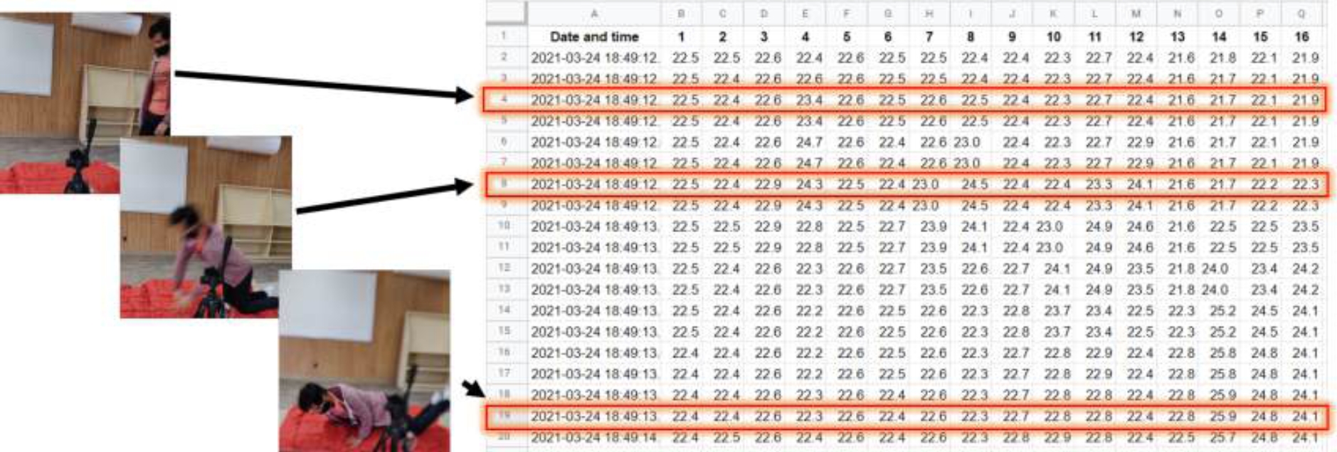
In each frame, 16 temperature values were captured and recorded at a specific time t (refer to Figure 1). These 16 frame temperatures are organized as a row in a CSV file, resulting in a total of 25 frames (rows) per file, as illustrated in Figure 2. The final dataset consists of 354 fall files and 899 non-fall files. The dataset is publicly available in the following repositoryfn.
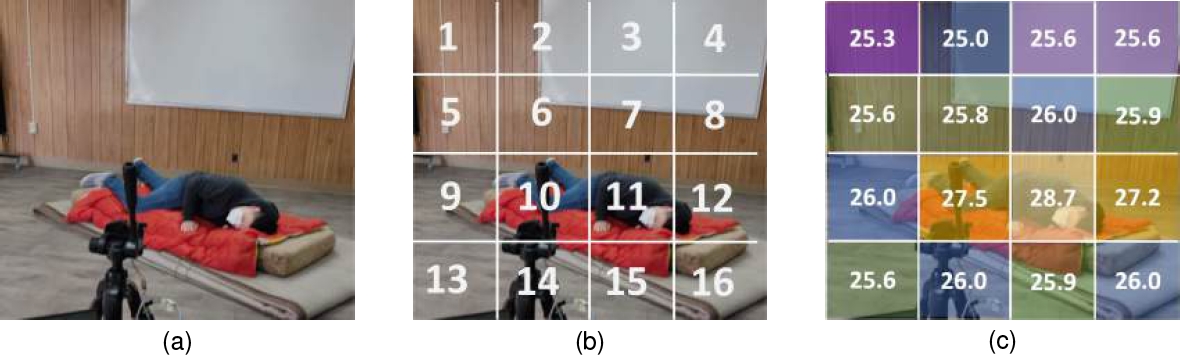
Fig. 1 Frame temperature readings: (a) Frame at time
3.3 Hyperparameters Tuning
The hyperparameter values are used to control the learning process of the ML model. Despite using the same training data, varying hyperparameter values lead to distinct trained models. The process of selecting the most effective combination of hyperparameter values is referred to as hyperparameter tuning and holds significant importance in attaining high model performance [30].
Unfortunately, there is not a one-size-fits-all set of optimal hyperparameters for all problems, and evaluating different combinations of hyperparameter values is computationally expensive. Nevertheless, hyperparameter tuning strategies and commonly employed hyperparameter values exist that have proven successful in addressing similar problems. In our experiments, we employed the widely used grid-search strategy for hyperparameter tuning in Support Vector Machines and Random Forests.
This strategy involves systematically selecting various hyperparameter values and evaluating all possible configurations. The grid-search process was implemented using the GridSearchCV function provided by the Scikit-learn Python library. This approach allows for a comprehensive exploration of hyperparameter combinations to identify the most effective configuration for our specific experiments [22].
Due to the consideration of a larger number of hyperparameters in the CNN architecture, we employed the hyperband method for hyperparameter tuning [15]. The hyperband method extends the successive halving algorithm [10], and its process is outlined as follows: a set of n hyperparameter values is evaluated for all configurations using limited resources (e.g., dataset size, training time, number of epochs).
After evaluation, the configurations with the worst performance are discarded, and the process is iterated until only the best configuration remains. Unlike the successive halving algorithm, the hyperband method allocates a specific number of iterations for different configurations, focusing on promising candidates for more extensive evaluations. In our work, hyperband tuning was implemented using the Keras hyperparameter tuning library [21]. Table 1 outlines the values considered for hyperparameter tuning in each machine learning model.
Table 1 Hyper-parameter values for each ML model
| Hyper-parameter | Selection |
| CNN | |
| layers | 1, 2,3 |
| nodes (1st layer) | [:256, step=32] |
| nodes (2nd layer) | [:256, step=32] |
| nodes (3rd layer) | [:256, step=32] |
| pooling | average, maximum |
| fully connected | [:256, step=16] |
| activation function | ReLU, tanh |
| optimizer | SGD, Adam |
| learning rate | [-5:10-2, step=×10] |
| batch size | 1, 16, 32, 64 |
| SVM | |
| C-value | [-2:103, step=×10] |
| gamma | [-4:1, step=×10] |
| kernel | Linear, polynomial, radial, sigmoid |
| RF | |
| n_estimators | 30, 50, 100, 300 |
| max_depth | None, 3, 10, 30, 50, 100 |
| min_samples_leaf | 3, 5, 10, 30 |
| max_features | None, auto, sqrt, log 2 |
| bootstrap | True, False |
4 Results and Discussions
Following hyperparameter tuning, the best configurations for the three machine learning models are described as follows. For the SVM classifier, the best hyperparameter configuration was {
For the RF model, the best hyperparameter configuration was {non-bootstrap, max_depth=50, min_samples_leaf = 3, n_estimators = 100}.
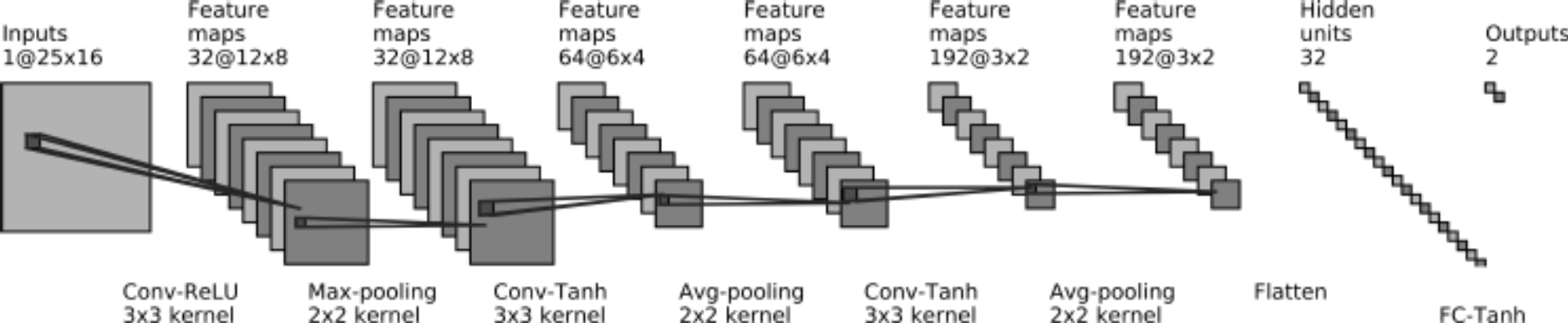
Lastly, for the CNN architecture, we obtained a three-convolutional layer network followed by two fully connected layers. The first convolutional layer consists of 32 filters (3×3) with a ReLU activation function followed by a max pooling layer (2×2). The second and third convolutional layers consist of 64 and 192 filters (3×3), respectively, followed by an average pooling layer (2×2). After convolutional layers, a fully connected layer of 32 nodes and a tanh activation function were added.
The output layer has two nodes and a softmax activation function. Figure 3 shows the CNN architecturefn. These configurations represent the best-performing settings after thorough hyperparameter tuning for each respective machine-learning model.
The training of the CNN architecture involved the utilization of the cross-entropy loss function and the Adam optimization algorithm [13]. The model was trained with a learning rate set to 10-3 and a batch size of 16 throughout 30 epochs. These parameters were chosen to optimize the training process and achieve effective learning for the given dataset.
The performance results obtained by the models were assessed through repeated 3×10-fold cross-validation [11]. The evaluation employed standard performance metrics for machine learning models [11], including Accuracy (ACC), Balanced Accuracy (BACC), and Area Under the Receiver Operating Characteristic Curve (AUC-ROC). These metrics offer a comprehensive evaluation of the overall method performance.
Table 2 shows the average results of the evaluated ML techniques alongside related literature works. It is evident that the CNN, SVM, and RF models exhibit robust capabilities in distinguishing between falls and non-fall events, achieving performances consistently above 95% across all metrics.
Table 2 ML results
| Model | ACC | BACC | AUC-ROC |
| Mashiyama | 0.958 | – | – |
| Taniguchi | 0.955 | – | – |
| CNN | 0.96 | 0.95 | 0.99 |
| SVM | 0.99 | 0.98 | 0.99 |
| RF | 0.99 | 0.99 | 0.99 |
In comparison to the works of Mashiyama et al. [17] and Taniguchi et al. [26] works, our evaluated machine learning models demonstrated superior performances, exceeding 96% accuracy with only one sensor and a lower sensor resolution.
Notably, the RF classifier achieved outstanding performance, reaching up to 99% for ACC, BACC, and AUC-ROC. Moreover, Figure 4 illustrates that the RF model incurred only four errors, primarily misclassifying non-fall data as fall data.
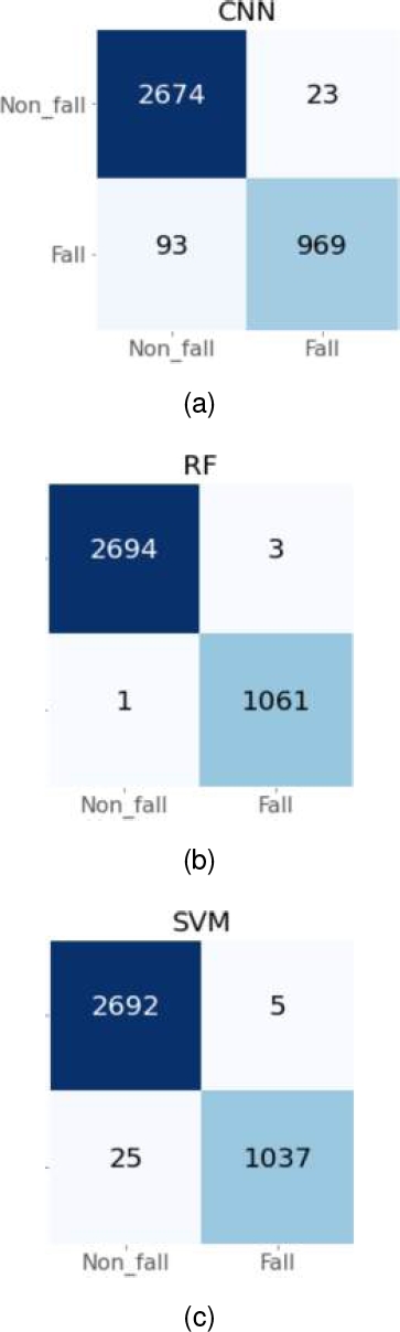
Importantly, misclassifying a non-fall event as a fall event is often considered less critical than the opposite scenario. This emphasizes the effectiveness of the RF model in minimizing errors and underscores its potential as a reliable fall detection solution.
5 Conclusion and Future Work
This work addresses the problem of elderly fall event detection using a thermal sensor and machine learning techniques. Unlike other devices, the thermal sensor is less invasive, has no need to be manipulated, and maintains privacy. Additionally, the sensor’s low resolution opens up possibilities for embedded applications, enhancing its versatility in various contexts.
The experimental dataset utilized in this study was generated by students through simulations of both fall and non-fall events, during which a thermal sensor recorded room temperatures. The captured data for each event was subsequently stored in a CSV file. The compiled dataset comprises a total of 1,253 CSV files, consisting of 354 fall events and 899 non-fall events. Each file is structured with 25 rows (frames) and 16 columns, representing the recorded room temperatures during the respective events.
For the fall event detection, we selected three well-known supervised machine learning models that have shown outstanding performance for several machine learning tasks: SVM, RF, and CNN. The experimental outcomes affirm the efficacy of the CNN, SVM, and RF models in effectively distinguishing between fall and non-fall events. Notably, the random forest classifier demonstrated the most favorable results in 3×10-Fold cross-validation, with merely four errors. This underscores the remarkable detection capabilities achievable with just one sensor.
The findings highlight the potential of leveraging these machine-learning models for reliable and efficient fall detection using minimal sensor resources. In future research works, it would be beneficial to incorporate more complex scenes during the training stage, encompassing scenarios involving multiple individuals or pets.
This approach aims to enhance the robustness of the fall detection system by exposing it to a broader range of environmental conditions. By training the system on diverse and challenging scenarios, it can develop a more comprehensive understanding of potential fall events in real-world settings, thus improving its reliability and applicability across various contexts.

