1 Introduction

Optimization problem-solvers aim to find solutions that minimize or maximize at least one objective function (OF). So broadly speaking, optimization problems can be divided according to the number of OF that the solver handles to obtain the optimal values; hence, there are two big groups: In the first one, the problem-solver use only one objective function, thus we are dealing with a single objective optimization problem (SOOP).

In the second group, the problem-solver compromises the solutions to satisfy in the best possible way more than one OF; these kinds of problems belong to a class known as multiobjective optimization problems (MOOP). MOOPs are harder to solve than SOOPs; consequently, through history, there have been many proposals focused on reducing obstacles in the diverse facets of the problem solver, i.e., the algorithms or methods.

Some ideas of the first proposed methods referred to as classical methods, to distinguish them from metaheuristic-based methods were classified by Miettinen in [¹] as follows:

The no-preference methods use a heuristic to find a single optimal solution without assuming any information concerning the importance of the objectives. In contrast, posteriori methods use preference information about each objective and generate a set of Pareto optimal solutions [²].

The a priori methods usually find a preferred Pareto optimal solution using information concerning the preferences of objectives [³]. Interactive methods work with preference information progressively along the optimization process [⁴].

Three of the more popular classical methods are the weighted sum approach (WSA), the Benzon method [⁵], and the normal boundary intersection (NBI) [⁶, ⁷].

Regarding metaheuristic methods, Shaffer proposed to solve a MOOP using a genetic algorithm to find a solution in each run of a WSA [⁸]. A different way to deal with a MOOP is with a multiobjective optimization evolutionary algorithm (MOOEA), which find multiples solutions in the Pareto front in each run.

MOOEA has significantly grown since the Pareto dominance concept was proposed by Goldberg [⁹] and still being the preferable option to obtain a set of optimal viable solutions. The use of the NBI presents several significant drawbacks; some of them are:

A way to deal with the difficulty of the constraint equation in the NBI is combining it with a metaheuristic algorithm and penalize the solution that did not fulfill the constraints like the proposed by Zhang and Li in the MOEA/D [¹²]. The MOEA/D decompose the objective space of a MOOP in N subproblems with different weight vectors, to solve these subproblems, the authors reported experiments with three classic methods: The Weighted Sum Approach, the Tchebycheff Approach, and a Boundary Intersection (BI) Approach.

Similarly, in [¹³], the NBI and the Tchebycheff method are used to guide the search in the neighborhood of the MOEA/D; in this algorithm the classic method and the evolutionary algorithms works together to solve a MOOP; however, the search direction needs to be defined yet.

Another weakness of the MOEA/d is that the recombination operators affect their performance, to solve this in [¹⁴] Luo et al. proposed the genetically hybrid differential evolution strategy for recombination that use one mutation strategy focused on the diversity and another focused in convergence.

The problems of the quick convergences and the loss of the diversity affect also the particle swarm optimization algorithms, to avoid this a fusion learning strategy that improved the leadership selection strategy is presented in [¹⁵]. The Radial Boundary Intersection based decomposition with an Interior-Point method (RBI-IP) [¹⁶] is an algorithm that also uses the NBI.

This algorithm decomposes the objective space in N sub-problems, each of one is solved to find the closets solution to the reference point on the respective radial line, these solutions are found using the interior point method.

Another improvement of the NBI is presented by Cui et al. [¹⁷] they use the adaptive weight sum, the adjust uniform axes method and Mahalanobis distance to get a wide and uniform distribution of the Pareto Frontier. In this paper, we propose the Normal Attractor Intersection (NAI) method and the Normal Attractor Intersection multi-objective particle swarm optimization (NAImopso).

The first one is a method inspired by the NBI [⁶], the improved NBI [¹⁸], and the Tchebycheff approach. The NAI avoids the a priori definition of the search direction and the equality constraints; a set of attractors that cover the entire Pareto Front are used, minimizing the normal distance to one of these attractors, then a Pareto point is obtained.

The second one is a multiobjective optimization algorithm based on decomposition; we used it to prove the ability of the NAI to obtain the Pareto front. It guides the search, and the structure of the randomly selected neighbors-particle swarm optimization (RSN-PSO) proposed in [¹⁹] adapted to deal with multiobjective optimization is used to generate new solutions.

We compare our proposal against four multiobjective metaheuristics based on the PSO that are in the state-of-the-proposals; they are the pccsAMOPSO [²⁰] and the KGMOPSO [¹⁵]. The evaluation was achieved using three well-recognized indicators used as performance metrics; they are the hypervolume indicator, the coverage, and the ε-indicator. The experimental results showed that solutions obtained with the NAImopso were better than the solutions obtained with the other algorithms with it was compared.

The rest of this paper is organized as follows: Section 2 describes the theory of the NBI to understand the inspiration of the NAI. Sections 3 and 4 introduce the proposed NAI and NAImopso respectively. Section 5 reports the experimental results. Section 6 concludes the paper.

3 Normal Attractor Intersection

The algorithms that transform a MOOP into a single-objective optimization problem are easier to implement and use than the Pareto dominance-based algorithms, but the preference of each objective needs to be defined as a priori in a weight vector.

The NBI has advantages over other classical methods that obtain solutions with a better distribution on the Pareto front; in contrast, it converts a MOOP in a set of SO optimization problems with equality constraints that could be hardest to solve than the MOOP. In gradient-based methods, the Karush-Kuhn-Tucker condition is used to deal with equality constraints. In evolutionary algorithms, it is common to penalize the individuals that do not satisfy the constrains; an example is the penalty-based boundary intersection (PBI) approach [¹²].

In the NBI, the search direction needs to be defined. If the objective space has a convex region and a non-convex region, the direction needs to change. In [¹⁸] use the CHIM_MOD, a dashed line over the axis f1(x), the problem of maximize t in the original NBI is changed to minimize t,and the search direction is not dependent of the objective space form, in [¹⁸] only are reported results for bi-objective problems.

In our proposal, the Normal Attractor Intersection (NAI) method, the normal vector direction to CHIM, does not have to be defined a priori, which is an advantage over the NBI. The above advantage is due to the NAI uses a set of attractors {β1,β2,…,βN}, where βn∈RM, instead of using the CHIM. The attractors enclose the entire Pareto front, as shown in the ¡Error! No se encuentra el origen de la referencia., so the set of attractors is a set of points distributed in M lines parallel to the objective axis.

Equation (9) allows to obtain each element βmn of an attractor point βn=[β1n,β2n,…,βMn]T parallel to the i objective axis. Where wn∈[0,1] is the weight of the attractor point n. The equation (9) only applies for m=i. For m≠i, βmn=zm*, this is to ensure that the attractor point n is parallel to the objective axis i, and it covers all the Pareto front:

Using the set of attractors, the NAI convert a MOOP in N subproblems of one objective were to obtain a point in the Pareto front the value of the normal distance tn between the objective space and the attractor βn is minimized like is shown in the Fig. 2, so using this approach a n subproblem of the MOOP is solving as follows:

Minimize:

Subject to:

where n^ is the normal vector obtained by the equation (14) and e is a vector of ones:

Fig. 1 Graphical representation of the CHIMmod that cover the entire Pareto front in (a) the zdt1 problem, and (b) zdt3 problem 

Fig. 2 Graphical representation of the NAI in the zdt1 problem 

The previous approach has the same problem of the NBI and the improved NBI; the equality constraints still need to be satisfied.

For these reasons, we propose to use a method like Tchebycheff decomposition, but instead of minimizing the maximal distance between a point and the ideal vector multiplied by a weight, we minimize the maximal distance between a point and an attractor.

To ensure that the obtained Pareto optimal point is parallel to the attractor, the angle α penalize the solution, while α is closer to zero, the point is closer to the normal, so atnis an image of tn in the previous approach, this new method is called Normal Attractor Intersection NAI, so a MOOP is decomposed in n subproblems, each of one is solved as follow:

Minimize:

Subject to:

where α=atan(fi(x)−βinfk(x)−βkn)>0 is a variable to keep the solution normal to the i axis, and fk(x)−βkn is the distance of the solution in any k≠i axis to the attractor point.

4 Normal Attractor Intersection Based Multi-objective Optimization Using Particle Swarm Optimization NAImopso

The NAImopso is a PSO based algorithm that decomposes the objective space of a MOOP in 𝑁 subproblems; each one is solved using the NAIB with different attractors. The fitness of each particle is obtained evaluating one subproblem, so the size of the swarm is N too; each particle p has an attractor βp and a neighborhood Bp, where Bp is a set with the τ closets attractors to βp, for each

particle p a new subswarm is generated with τ particles that are evaluated with one of the attractors in Bp.

To preserve the diversity and ensure to obtain a good approximation to the Pareto front, the particles in NAImopso learn from Sbest which is the particle with the best fitness in the subswarm and from RSNbest that is the best particle in a randomly selected neighborhood of size ns from the subswarm. The use of the RSNbest was proposed in [¹⁹] were to avoid the stagnation used the renewelGap parameter, which is the maximal number of iterations without update the Sbest.

The position and velocity of each particle i in the subswarm is updated using the equations (18) and (19) where c1, c2 and c3 are the coefficients, Sbestid(t) is the decision variable d of the particle in the subswarm with the best fitness, and RSNbestid(t) is the value of the best particle in the random selected neighborhood:

To calculate the fitness of the new position xi(t+1) of each particle i first each objective function is evaluated with this position, F1(xi(t+1)), F2(xi(t+1)), …, FM(xi(t+1)), then a scalar fitness is calculated using the NAIB with the attractor βi∈βp previously assigned.

If the fitness of the new position is minimal, assuming that it is a minimization problem, the Pbest fitness and the Sbest fitness are updated. The NAImopso pseudocode is shown in Algorithm 1; the output is the Pbest of each particle, i.e., N points distributed in the Pareto front.

Algorithm 1 NAImopso algorithm 

5 Experiments

To test the performance of the proposed NAImopso the two objective benchmark function ZDT1, ZDT2, ZDT3, ZDT4 and ZDT6 [²²] and the three-objective function DTLZ2 [²³] were used. We compared the results against other state-of-the-art multiobjective metaheuristics based on the PSO; they are the pccsAMOPSO [²⁰] and the KGMOPSO [¹⁵]. In the tests performed with the NAImopso, the number of particles used was N=100. This number is equal to the numbers of attractors; for each one, we have a point in the Pareto front.

The number of particles in the subswarm of each particle was τ=40; the size of the subswarm was selected according to the most common size reported in the literature; we obtained good results in performance and computational time with this size.

A value of the size of the neighborhood that can obtain a good balance between exploration and exploitation, according to [¹⁹] is ns=5. The parameters of the PSO were set as X=0.7298 and c1=c2=c3=2.05.

The experiments were running in a computer with the processor Intel(R) Core (TM) i7-8650U CPU @ 1.90GHz and 16 Gb of RAM. The algorithm was implemented in C++, the mean execution time for each run was 165.21 seconds, the faster time was 44.0 seconds and the slower was 239.0 seconds.

The inverted generational distance (IGD) is used to compare the performance of the NAImopso, the IGD is a measure between the solution S and a set of targeted points on the Pareto Front R [²⁴]. The IGD is calculated as follows:

where d(ri,sj) is the euclidean distance between the solution S∈S1,S2,…,Sμ and the targeted point R∈R1,R2,…,R|R|.

We executed the NAImopso 30 times to obtain the mean and the standard deviation of the IGD. The results and comparisons are shown in the Table 1, we can observe that the NAImopso obtained better results than other algorithms when optimizing the ZDT1, ZDT2, and DTLZ2 problems.

The NAImopso does not use any non-dominated method, because of that for multimodal problems as the ZDT4 and non-uniform (ZDT6) all the solution is not in the Pareto Front, but with a non-dominated method in the last population we can remove the dominated solutions. There are different metrics (indicators) to evaluate the output quality or the different evaluated algorithms [²⁵, ²²]. In this work, we chose to perform the evaluation using the next three metrics: the hypervolume indicator S(X′) [²⁶], the additive epsilon indicator Iϵ+(X′,X″) [²⁶], and the coverage C(X′,X″) metric [²⁷].

The hypervolume indicator is proportional to the distribution of the solutions $X'$ in the Pareto front; hence this metric captures the proximity of the solution set to the true Pareto front as well as its distribution in the objective space, better solution sets are those with the larger values. The additive epsilon indicator measures the smallest distance by which a Pareto approximate front (X′), obtained by one algorithm, must be shifted in the objective space to dominate another Pareto approximate front (X″) obtained by another algorithm.

It provides a relative measurement that expresses the minimum necessary value of ϵ that should be added to the solutions $x′i∈X′, and then they dominate all solutions in X″ [²⁸]; the smaller values represent the best solutions.

The coverage C(X′,X″) indicator describes the percentage of solutions in the set X′ that dominates the solutions in the set X″; in this case, it is desirable to get big values from this indicator [²⁷]. Table 2 shows the results of these evaluations. In the table, we can observe that the hypervolume value of the solutions obtained with the NAImopso S(A) is better for the ZDT2 and ZDT3 problems.

In the four problems, the solutions of the NAImopso cover a larger percentage of the solutions of the MOEA/d C(A,B); conversely, the MOEA/d cannot cover the range of solutions obtained with the NAImopso C(B,A). Additionally, according to the additive epsilon indicator, the NAImopso is better in the ZDT2 problem. In the Fig. 3 is shows the Pareto front of the ZDT1, ZDT2, and ZDT3 problems, the non-dominated points obtained with the MOEA/D and the Pareto candidates obtained with the NAImopso.

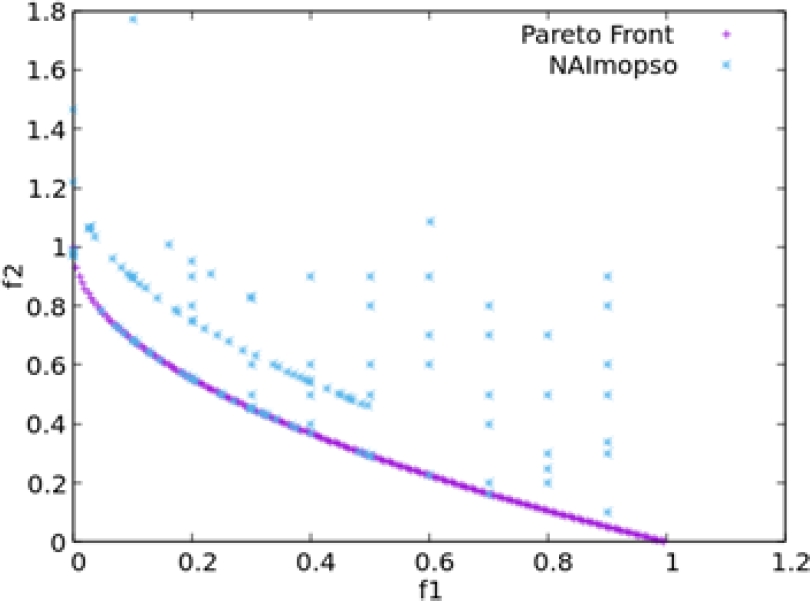
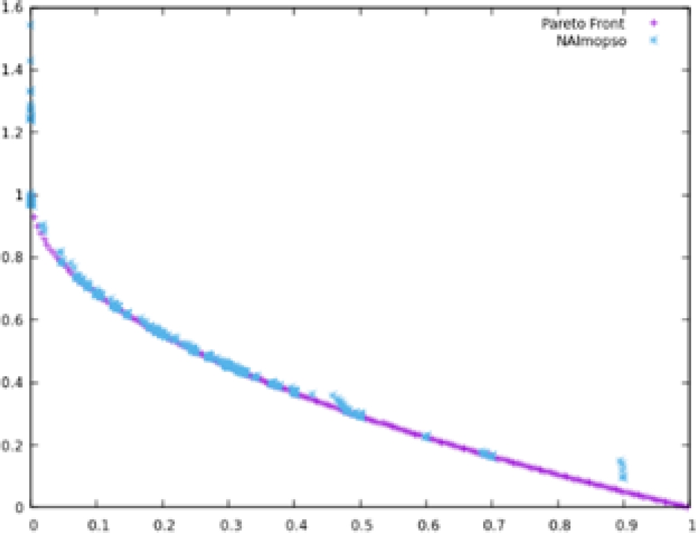
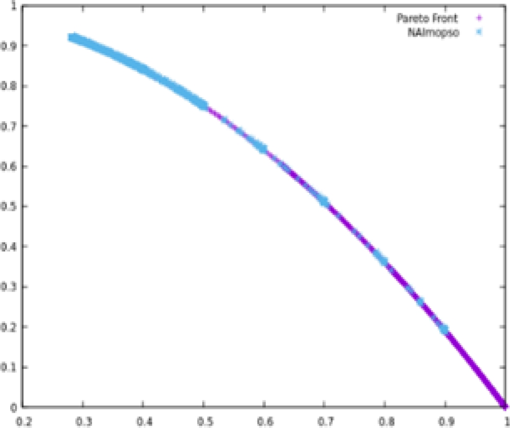
Fig. 3 We indicated the True Pareto front using a `-', the Pareto approximate front obtained with the MOEA/D with an 'x', and the Pareto approximate front obtained with the NAImopso with an '*'. (a) Pareto front of the ZDT1. (b) Pareto front of the ZDT2. (c) Pareto front of the ZDT3 

In Fig. 3 (a) and Fig. 3 (b) show the results obtained for the ZDT1 and ZDT2 functions, we can observe that the solutions of the NAImopso have a better distribution on the Pareto front than MOEA/d, the above can be corroborated because the value of the 𝑆 metric is higher as can be seen in Table 2 which also shows that the coverage of the NAImopso over the MOEA/d is therefore higher. In Fig. 3 (c) we can observe that the solution of the NAImopso is closer to the Pareto front but to there are a set of points that no are non-dominated solutions.

In Fig. 4 (a) the Pareto front of the DTLZ2 function, the non-dominated points obtained with the MOEA/D, and the Pareto candidates obtained with the NAImopso are shown, the results of the NAImopso are on the Pareto front but as can see in the Fig. 4 (b) are only the solutions normal to the axis and not the entire Pareto front.

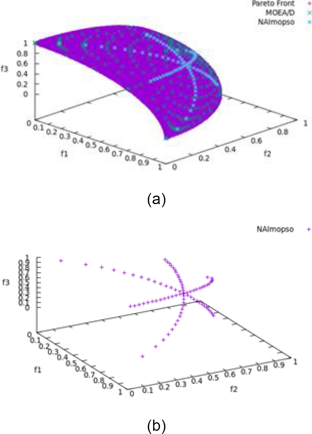
Fig. 4 Non-dominated and Pareto front candidates obtained with the MOEA/D and the NAImopso for DTLZ2 function. (a) Pareto front of the DTLZ2. (b) Pareto front of the DTLZ2 obtained with the NAImops 

For the ZDT4 problem due to it is multimodal, in the final solution there are non-dominated and dominates solutions, as shown in the Fig. 5, in the solution of the NAImopso we use the algorithm proposed by Mishra and Harit [²⁸] to find the non-dominated solutions, the final population is the show in the Fig. 6. For the ZDT6 problem, we also used the Mishra and Harit algorithm to keep only the non-dominated solutions, as shown in Fig. 7.

Fig. 5 Final solutions of the NAImopso for the ZDT4 problem 

Fig. 6 Solutions of the NAImopso for the ZDT4 problem after eliminated de dominated solutions 

Fig. 7 Solutions of the NAImopso for the ZDT6 problem after eliminated de dominated solutions 

6 Conclusion

In this paper, we proposed the NAI and the NAImopso methods; they provide a synergetic combination of a classical method and a bio-inspired algorithm that performs better than the MOEA/d. The combination of methods allows obtaining good results without using the non-dominated search that uses most of the Evolutionary algorithms. The solutions are Pareto candidates, and we do not use any strategy to ensure that the solutions are Pareto points; however, the decision-maker could apply a non-dominated method or evaluate only the selected solutions.

For problems with three objectives, a good representation of Pareto front is obtained which in real multi-objective optimization problems could facilitate the work for the decision-maker, although the solutions are not distributed in the entire Pareto front. We compared the NAImopso with other PSO multi-objective algorithms, such as the pccAMOPSO, cdAMOPSO, clusterMOPSO, and the pdMOPSO. The IGD metric was used to evaluate the different algorithms. The NAImopso obtained better solutions when optimizing the ZDT1, ZDT3, and DTLZ2 problems. In the case of the ZDT2, the results of NAImopso were as good as those obtained with the other algorithms.

Independently of the NAImopso, the NAI can be used with other multi-objective algorithms to guide the search. Moreover, it can be used in preference algorithms and to optimize problems with many-objectives. Also, to improve the capacity to find better non-dominated solutions we can prove to add dynamic adjustment of the parameters with fuzzy logic like the proposed in [²⁹] or use NAImopso with a Bacterial foraging optimization (BFO) as is described in [³⁰].

References

1. Miettinen, K. (1998). Nonlinear multiobjective optimization. International Series in Operations Research and Management Science, Springer US, Vol. 12, pp. 257–298. DOI: 10.1007/978-1-4615-5563-6. [ Links ]
2. Stadler, W. (1979). A survey of multicriteria optimization or the vector maximum problem, part I: 1776–1960. Journal of Optimization Theory and Applications, Vol. 29, No. 1, pp. 1–52. DOI: 10.1007/bf00932634. [ Links ]
3. Rivera, G., Coello-Coello, C. A., Cruz-Reyes, L., Fernandez, E. R., Gomez-Santillan, C., Rangel-Valdez, N. (2022). Preference incorporation into many-objective optimization: an ant colony algorithm based on interval outranking. Swarm and Evolutionary Computation, Vol. 69, pp. 101024. DOI: 10.1016/j.swevo.2021.101024. [ Links ]
4. Rivera, G., Cruz-Reyes, L., Fernandez, E., Gomez-Santillan, C., Rangel-Valdez, N. (2023). An interactive ACO enriched with an eclectic multi-criteria ordinal classifier to address many-objective optimisation problems. Expert Systems with Applications, Vol. 232, pp. 120813. DOI: 10.1016/j.eswa.2023.120813. [ Links ]
5. Benson, H. P. (1992). A finite, nonadjacent extreme-point search algorithm for optimization over the efficient set. Journal of Optimization Theory and Applications, Vol. 73, No. 1, pp. 47–64. DOI: 10.1007/bf00940077. [ Links ]
6. Das, I., Dennis, J. (1996). Normal-boundary intersection: An alternate method for generating pareto optimal points in multicriteria optimization problems. Contractor, no. 96, pp. 38. [ Links ]
7. Ganesan, T., Vasant, P., Elamvazuthi, I. (2013). Normal-boundary intersection based parametric multi-objective optimization of green sand mould system. Journal of Manufacturing Systems, Vol. 32, No. 1, pp. 197–205. DOI: 10.1016/j.jmsy.2012.10.004. [ Links ]
8. Schaffer, J. D. (1985). Some experiments in machine learning using vector evaluated genetic algorithms, PhD Thesis. [ Links ]
9. Goldberg, D. E. (1989). Genetic algorithms in search, optimization and machine learning, 1st ed. Addison-Wesley Longman Publishing Co., Inc. [ Links ]
10. Logist, F., van-Impe, J. (2011). Novel insights for multi-objective optimisation in engineering using normal boundary intersection and (enhanced) normalised normal constraint. Structural and Multidisciplinary Optimization, Vol. 45, No. 3, pp. 417–431. DOI: 10.1007/s00158-011-0698-8. [ Links ]
11. Dias-Lopes, L. G., Brito, T. G., Paiva, A. P., Peruchi, R. S., Balestrassi, P. P. (2016). Robust parameter optimization based on multivariate normal boundary intersection. Computers and Industrial Engineering, Vol. 93, pp. 55–66. DOI: 10.1016/j.cie.2015.12.023. [ Links ]
12. Zhang, Q., Li, H. (2007). MOEA/D: A multiobjective evolutionary algorithm based on decomposition. IEEE Transactions on Evolutionary Computation, Vol. 11, No. 6, pp. 712–731. DOI: 10.1109/tevc.2007.892759. [ Links ]
13. Rubio-Largo, Á., Zhang, Q., Vega-Rodríguez, M. A. (2014). A multiobjective evolutionary algorithm based on decomposition with normal boundary intersection for traffic grooming in optical networks. Information Sciences, Vol. 289, pp. 91–116. DOI: 10.1016/j.ins.2014.08.004. [ Links ]
14. Luo, N., Lin, W., Jin, G., Jiang, C., Chen, J. (2021). Decomposition-based multiobjective evolutionary algorithm with genetically hybrid differential evolution strategy. IEEE Access, Vol. 9, pp. 2428–2442. DOI: 10.1109/access.2020.3047699. [ Links ]
15. Li, W., Meng, X., Huang, Y., Mahmoodi, S. (2021). Knowledge-guided multiobjective particle swarm optimization with fusion learning strategies. Complex and Intelligent Systems, Vol. 7, No. 3, pp. 1223–1239. DOI: 10.1007/s40747-020-00263-z. [ Links ]
16. Datta, S., Ghosh, A., Sanyal, K., Das, S. (2017). A radial boundary intersection aided interior point method for multi-objective optimization. Information Sciences, Vol. 377, pp. 1–16. DOI: 10.1016/j.ins.2016.09.062. [ Links ]
17. Cui, J., Pan, J., Wang, S., Okoye, M. O., Yang, J., Li, Y., Wang, H. (2022). Improved normal-boundary intersection algorithm: a method for energy optimization strategy in smart buildings. Building and Environment, Vol. 212, pp. 108846. DOI: 10.1016/j.buildenv.2022.108846. [ Links ]
18. Siddiqui, S., Azarm, S., Gabriel, S. A. (2012). On improving normal boundary intersection method for generation of pareto frontier. Structural and Multidisciplinary Optimization, Vol. 46, No. 6, pp. 839–852. DOI: 10.1007/s00158-012-0797-1. [ Links ]
19. Sun, W., Lin, A., Yu, H., Liang, Q., Wu, G. (2017). All-dimension neighborhood based particle swarm optimization with randomly selected neighbors. Information Sciences, Vol. 405, pp. 141–156. DOI: 10.1016/j.ins.2017.04.007. [ Links ]
20. Hu, W., Yen, G. G. (2015). Adaptive multiobjective particle swarm optimization based on parallel cell coordinate system. IEEE Transactions on Evolutionary Computation, Vol. 19, No. 1, pp. 1–18. DOI: 10.1109/tevc.2013.2296151. [ Links ]
21. Aghaei, J., Akbari, M. A., Roosta, A., Baharvandi, A. (2013). Multiobjective generation expansion planning considering power system adequacy. Electric Power Systems Research, Vol. 102, pp. 8–19. DOI: 10.1016/j.epsr.2013.04.001. [ Links ]
22. Zitzler, E., Deb, K., Thiele, L. (2000). Comparison of multiobjective evolutionary algorithms: empirical results. Evolutionary Computation, Vol. 8, No. 2, pp. 173–195. DOI: 10.1162/106365600568202. [ Links ]
23. Deb, K., Thiele, L., Laumanns, M., Zitzler, E. (2002). Scalable multi-objective optimization test problems. Proceedings of the Congress on Evolutionary Computation, Vol. 1, pp. 825–830. DOI: 10.1109/cec.2002.1007032. [ Links ]
24. Narukawa, K., Setoguchi, Y., Tanigaki, Y., Olhofer, M., Sendhoff, B., Ishibuchi, H. (2015). Preference representation using gaussian functions on a hyperplane in evolutionary multi-objective optimization. Soft Computing, Vol. 20, No. 7, pp. 2733–2757. DOI: 10.1007/s00500-015-1674-9. [ Links ]
25. Okabe, T., Jin, Y., Sendhoff, B. (2003). A critical survey of performance indices for multi- objective optimisation. The Congress on Evolutionary Computation, Vol. 2, pp. 878–885. DOI: 10.1109/cec.2003.1299759. [ Links ]
26. Zitzler, E., Thiele, L., Laumanns, M., Fonseca, C., da-Fonseca, V. (2003). Performance assessment of multiobjective optimizers: an analysis and review. IEEE Transactions on Evolutionary Computation, Vol. 7, No. 2, pp. 117–132. DOI: 10.1109/tevc.2003.810758. [ Links ]
27. Zitzler, E., Thiele, L. (1999). Multiobjective evolutionary algorithms: a comparative case study and the strength pareto approach. IEEE Transactions on Evolutionary Computation, Vol. 3, No. 4, pp. 257–271. DOI: 10.1109/4235.797969. [ Links ]
28. Mishra, K. K., Harit, S. (2010). A fast algorithm for finding the non dominated set in multiobjective optimization. International Journal of Computer Applications, Vol. 1, No. 25, pp. 46–54. DOI: 10.5120/460-764. [ Links ]
29. Kawano, Y., Valdez, F., Castillo, O. (2022). Fuzzy combination of moth-flame optimization and lightning search algorithm with fuzzy dynamic parameter adjustment. Computación y Sistemas, Vol. 26, No. 2, pp. 743–757. DOI: 10.13053/cys-26-2-4269. [ Links ]
30. Mathur, R. P., Sharma, M. (2023). A multi-objective task scheduling scheme GMOPSO-BFO in mobile cloud computing. Computación y Sistemas, Vol. 27, No. 2, pp. 477–488. DOI: 10.13053/cys-27-2-3953. [ Links ]
Received: February 28, 2024; Accepted: May 15, 2024
* Corresponding author: Josué Domínguez-Guerrero, e-mail: josue.dominguez@uacj.mx
Creative Commons License This is an open-access article distributed under the terms of the Creative Commons Attribution License