2.1 Optimization Problem

Optimization problems are prevalent across various fields, including engineering, logistics, finance, and artificial intelligence. These problems involve finding the optimal solution, often within complex constraints or large solution spaces [²⁰]. Traditional optimization techniques, such as linear programming or gradient descent, are effective for well-structured problems but frequently struggle with highly nonlinear, multi-modal, or combinatorial optimization challenges [⁶].

These conventional methods often encounter difficulties in identifying optimal solutions within a practical time frame. This is where metaheuristic methods become essential [⁴]. Metaheuristic methods encompass a class of optimization algorithms designed to tackle complex and computationally demanding optimization problems. Unlike deterministic approaches, metaheuristics rely on heuristic or rule-of-thumb strategies, avoiding explicit mathematical models [¹¹]. These algorithms explore solution spaces by adeptly balancing exploration to discover new areas of the landscape and exploitation to refine promising solutions.

The strength of metaheuristics lies in their adaptability and versatility, as they can be customized for various problem types and constraints. Additionally, they excel in solving real-world challenges where exact solutions are often impractical due to computational limitations [¹¹]. As technology advances and optimization problems become increasingly complex, the role of metaheuristics continues to expand, establishing them as indispensable tools for researchers and practitioners tackling real-world optimization issues.

Furthermore, quantum computing and recent proposals of quantum metaheuristics enhance the search process within the optimization landscape, opening new frontiers for addressing previously unsolvable problems [⁷].

The objective of optimization is to find the best possible solution, referred to as feasible solutions, which are measured using numerical functions, referred to as objective functions [¹⁵]. In the feasible solution set, the solution that yields the best objective function value is referred to as the optimal solution [⁵]. The formal definition is shown in:

Let f:X→ℝ be a function where X⊆ℝn n−dimensional in the form x=[x1,…,xn]T The aim is to:

where xj, j=1,…,n is identified as a decision variable, X refers to the feasible region and f is the objective function.

2.2 Quantum Computing Fundamentals

In quantum computing, the basic unit of information is a quantum bit commonly called a qubit, which has a form |ψ〉. Quantum computing mathematically represents qubits using Dirac notation, also referred to as bra-ket notation. For example, the ket |i〉=[1   i]T where i∈ℂ, and the ket |1〉=[0   1]T. A qubit is a linear combination of |0〉 and |1〉.

Bra and ket vectors are complex vectors within the Hilbert space, existing in a dual space. The notation 〈ψ| indicates a bra, which is the complex conjugate transpose of the ket vector |ψ〉. Hence, 〈ψ|=|ψ〉†, where the symbol † signifies the complex conjugate transpose operation.

In quantum computing, computational bases are fundamental for representing and manipulating information. The most common computational basis consists of the states |0〉 and |1〉, which are analogous to the binary bits “0” and “1” in classical computing. These states serve as the foundation for encoding and processing quantum information. The superposition principle in quantum mechanics permits a qubit to be in a linear combination of the two fundamental states, |0〉 and |1〉. This relationship is illustrated in Eq. 2:

In Eq. 2, α and β are complex numbers representing the probability amplitudes. When measuring a qubit, the likelihood of finding the qubit in state |0〉 or |1〉 is given by the square of the absolute value of α or β, respectively.

The normalization condition requires that the sum of these squares equals one: |α|2+|β|2=1. Classical computers use registers to store bits, likewise, quantum computers register and store qubits. Despite this, a quantum qubit register and a classical bit register differ in important ways.

Quantum bits, unlike classical bits, are in a superposition of states. This enables them to represent both “0” and “1” simultaneously, enabling quantum computers to handle multiple possibilities simultaneously. Furthermore, qubits are capable of becoming entangled, enabling a profound link between their states, despite being physically separated, which facilitates more efficient calculations. Eq. 3 represents a quantum register of size n mathematically. A tensorial product of two states (vectors) is represented by the symbol ⊗:

Quantum gates are fundamental in quantum computing. They function similarly to classical logic gates in traditional computing, enabling control over the state of one or more qubits. Thanks to quantum gates, quantum computers can carry out specific tasks much faster than classical computers, as quantum states can exist in superposition and be entangled [²⁷].

Operations can be performed on individual qubits or on groups of qubits, known as quantum registers. Some one-qubit quantum gates originate from the Pauli set. For instance, the X=[​10  ​01] gate, which induces rotations around the X-axis, and the Y=[​i0  ​0−i] gate, which causes rotations around the Y-axis.

Another significant one-qubit gate frequently used to bring a qubit into a superposition state is the Hadamard gate, H=12[​11   ​−11]. This superposition creates equal probabilities for the qubit to be in the |0〉 or |1〉 states, with the |1〉 state having a relative phase difference of π radians.

A one-qubit quantum gate acts on a quantum state as U|ψ〉, where U is a quantum operator such as the quantum gate H. For instance, applying the Hadamard gate H to the quantum state |0〉 yields H|0〉=12[​11   ​−11]=12[​11], which simplifies to H|0〉=|0〉+|1〉2. Another type of one-qubit gate is the rotation gate, which can be represented as:

In Eq.4, Rx(θ) represents a rotation about the x-axis, Ry(θ) denotes a rotation about the y-axis, and Rz(θ) indicates a rotation around the z-axis. The variable θ stands for the angle of rotation for each respective axis. As mentioned earlier, a quantum register consists of multiple qubits grouped together as a single entity.

Similar to single quantum gates, in a quantum register, a quantum gate denoted as Ur can operate on the quantum register state |ψr〉n of n qubits in the form Ur|ψr〉n. For example, the application of the H⊗2 gate (which is two Hadamard gates in parallel, i.e., H⊗H) on a two-qubit register |ψr〉2 is represented as H⊗2|ψr〉2, which can be expressed as:

In this case, S0…S3 represent the quantum states of |ψr〉2, and S′0…S′3 denote the quantum states that result from applying the quantum gate H⊗2 to the state |ψr〉n. In general, for a n-qubit state in the computational basis |0⋯0〉n, applying the Hadamard gate to each qubit results in:

This operation with the Hadamard gate is crucial, as many quantum algorithms use it as an initial state. It enables all the 2n orthogonal qubits in the basis states |0〉 and |1〉 to be placed into a superposition state with equal probabilities. In general, the procedure can be expressed as:

where x⊙z denote the bit-by-bit inner product of x and z.

Measurement plays a fundamental role in quantum mechanics, offering insights into physical observables and their associated probabilities. It is essential to understand that measuring a quantum system disturbs it, causing an irreversible change in its state. In quantum computing, measurement is particularly significant for retrieving the information encoded within the computational system. In the domain of quantum mechanics, a range of measurement models are utilized to illustrate the interaction between a quantum system and a measurement apparatus, as well as the acquisition of measurement outcomes [²¹].

A variety of measurement models are used such as the Projection Model, Expectation Value Model, State Collapse Model, Statistical Model, and Eigenvalue and Eigenspace Model.

The standard notation of measurements consists of a measurement operator represented as Mm, where m is used as an index for a possible measurement outcome. If state is |ψ〉, the probability of getting a measurement result m is as the following:

Upon obtaining this measurement, the subsequent state will be:

Quantum computing depends on measuring a group of qubits “in the computational basis”, which consists of the states |0〉 and |1〉. In this particular scenario, we consider the spin direction of individual qubits in the quantum memory register along the z-axis of the Bloch sphere, which traverses both the North and South poles of the sphere.

The results of these measurements indicate that each qubit is either aligned with the z-axis, with “spin-up”, or it is in opposition, with “spin-down”, which corresponds to state |0〉 and |1〉 respectively. If this measure is applied to each qubit in a quantum memory register comprising n-qubits, will be obtained one of 2n possible bit strings configurations.

The generation of different outcomes is contingent upon the superposition of each binary string configuration present in the register immediately before measurement. To illustrate this, let us consider an n-qubit quantum memory register which is in the normalized state ∑i=02n−1ci|i〉 (where |i〉 represents a bit-string).

There will be variability in the outcome depending on the magnitude of the amplitudes ci and whether it is making a full measurement (measuring all the qubits) or a partial measurement (measuring only a few qubits). The result will be |i〉, with a probability of |ci|2 for each state.

2.3 Quantum Genetic Algorithm

An evolutionary algorithm represents an optimization approach inspired by biological evolution, used to identify or approximate solutions to intricate problems spanning various disciplines [¹⁶]. These algorithms commence with a population of potential solutions, subjecting each to fitness evaluation via a predefined function.

Selection for reproduction is based on fitness, leading to the generation of new solutions through crossover and mutation. This iterative process unfolds across multiple generations [¹¹]. Our work focuses on Quantum Genetic Algorithms (QGAs) [⁹], which are rooted in Quantum-Inspired Genetic Algorithms (QIGAs) [¹⁹]. The two types of algorithms are grounded in quantum principles but have distinct implementation and computational frameworks. Quantum-Inspired Genetic Algorithms (QIGAs) are classical algorithms that run on conventional computers. They are inspired by quantum principles and seek to replicate quantum effects using classical computing methods [²³].

In contrast, QGAs are specifically created to operate on authentic quantum computers, exploiting the complete potential of quantum characteristics. They possess the capacity for substantial acceleration in solving certain problems, however, their practical utility is currently constrained by the early stage of quantum hardware development and limited accessibility.

The specific approach of this study is implementing a Quantum Genetic Algorithm (QGA) using two programming languages that allow connection to quantum computers via AWS. In MATLAB, the ‘quantum’ package developed in 2023 was used. For Python, the Amazon Braket library was utilized. It is important to mention that these tools also allow simulations to be run on personal computers.

As discussed in [¹⁸], we have customized QGA for execution on quantum computers. We take the proposal developed in [²²] where “qi characterizes a quantum system |ψi〉 that encompasses 2m simultaneous states, as expressed in Eq. 10. Here, m represents the genetic composition of each individual, and i signifies the population size”:

The outcome will produce a quantum population structured in the following manner:

As a result, in [²²], Algorithm 1 and Algorithm 2 were developed. The Algorithm 1 requires two elements: the total amount to the evolution of population, i.e., generations, g, and the population size sp→i. In more detail on line 2, the generation number t is adjusted to 0.

Algorithm 1 Quantum genetic algorithm (QGA) 

Algorithm 2 Update of the QGA 

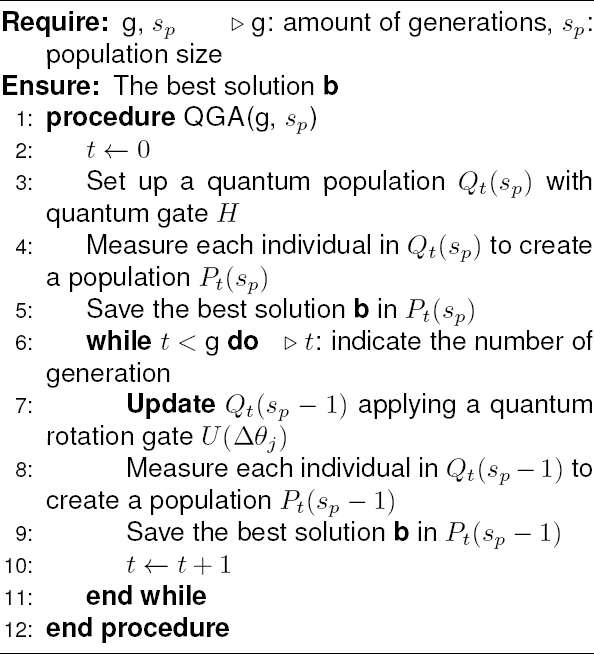
In line 3, we applied the quantum Hadamard gate to all the qubits, as defined in Eq. 7 to produce equal chance distributions for all potential individuals. In line 4, we obtain a classical population by measuring all individuals in the current population. In line 5, we store the best solution in the current population in “b”.

The while-loop, spanning from lines 6 to 10, runs continuously as long as the generation counter remains less than the maximum number, indicated as “g”. The process involves generating a new quantum population using the best solution “b” in line 7, followed by an update using Algorithm 2. A new classical population is then formed by measuring the individuals obtained in line 7 and line 8. In line 9, the best solution from the entire process is saved as “b”. Additionally, the generation counter is incremented at the end. The mutation is applied using the Ry gate, which consists of two parameters: the qubit of the i−th individual to which a certain rotation will be applied, and the degrees of rotation, assigned according to Table 1.

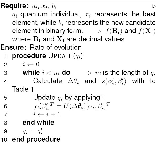
In [²²] explained that “ Algorithm 2 provides the required rotation angle that will eventually modify the amplitude probability to change individual qubits of the quantum chromosomes.

The algorithm relies on Table 1 to select the appropriate angle for its use in Eq. 12; this updates the corresponding qubit in the quantum chromosome”. The original strategy proposed in [¹⁰] to rotate the angle was modified as shown in Table 1:

For example, the way that we adapted the quantum inspiration was to take only the i−jth values and compare them, assigning a rotation based on said comparison, trying to ensure convergence towards a better individual. Suppose you have the best individual bi=10111110011 and the new individual obtained is xi=10110110110 plus their respective decimal values are Xi and Bi. If we will be taken xij=1 and bij=1, with i=1 and j=1. f(Xi) and f(Bi) are compared, using the Table 1, if f(Xi)≥f(Bi), it will assign Δθi=0.025π otherwise 0.005π.

3.1 Implementation of QGA on Quantum Device in AWS

Referring to the design explained in Section 2.3, the resulting quantum circuits are depicted in Figure 1. For the first quantum population, we applied the Hadamard quantum gate described in Eq. 7. To achieve the quantum mutation and crossover processes, we used the Ry(θ) quantum gate described in Eq. 12.

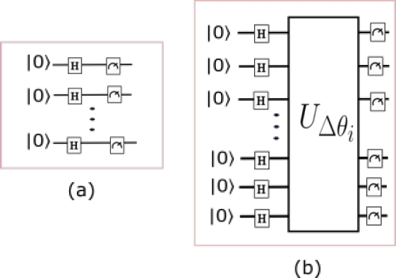
Fig. 1 The functions of the QGA are illustrated in the following diagram. (a) The quantum circuit for initializing the first population. (b) The quantum circuit for mutation and crossover operators. Figures taken from [³,²²] 

The characteristics of QGA are taken from [²²] where is used an array of 11 qubits to correspond to a single quantum chromosome. The population is constituted of 10 individuals.

A sequence of m=11 qubits is defined as a quantum chromosome qi, where i≤10. Therefore, we work with size chains of 11, each containing 10 elements. The precision was determined by the number of qubits available. In this case, 11 qubits were utilized. Among the devices listed in Table 2, only the Harmony from IonQ was accessible for MATLAB.

For Python, in addition to the Harmony device, Aria-1 was also available. The domain was chosen for values of x between [0.00, 127.00]. To ensure consistency in both implementations, a quantization method was employed to obtain decimal values, and they were represented with 4 decimal places after the decimal point.

The implementation of MATLAB with a specific quantum device is facilitated by the development of a library called ‘quantum’, which was introduced in 2023. The connection procedure is initiated through the command exemplified in Code3.1. It is noteworthy that the establishment of this connection necessitates the creation of an Amazon Web Services account. This applies to both Python and MATLAB, although the process differs for each.

loadenv ( ’ awsAccount.env ’ )

region = ” us−east −1 ” ;

bucketStoragePath = ” s3://amazon−braket −name

     Bucket / nameFolder / ” ;

deviceARN= ” arn : aws : braket : us−east − 1 : : device /

     qpu / ionq / Harmony ” ;

device = quantum . backend . QuantumDeviceAWS

     (devARN, Region=region , S3Path=

     bucketStoragePath ) ;

% Quantum c i r c u i t example

qcExample = quantumCircuit ( HGate ( 1 ) ) ;

taskExample = run ( qcExample , device ) ;

wait ( taskExample ) ;

measure = fetchOutput ( taskExample ) ;

% The next line shows r e s u l t s in a table from

t a b l e ( measure . Counts , measure . MeasuredStates ,

     VariableNames =[ ” counts ” , ” States ” ] )

One of the differences between MATLAB and Python, as demonstrated in Code 3.1, is that Python requires only a single line of code to set the session values and select the quantum device after installing the Amazon Braket library. An example is shown in Code 3.1.

#Required packages

! pip i n s t a l l amazon−braket −sdk

! pip i n s t a l l boto3

! pip i n s t a l l −−upgrade amazon−braket −sdk

! pip i n s t a l l −−upgrade amazon−braket −schemas

from boto3 import Session

from braket . aws import AwsDevice , AwsSession

from braket . c i r c u i t s import C i r c u i t

from braket . s i m u l a t o r import BraketSimulator

#Simulator

from braket . devices import LocalSimulator

# Use the awsAccount name _and_ region

session=Session (

aws_access_key_id= ’ ID awsAccount ’ ,

aws_secret_access_key= ’ access_key_awsAccount ’ ,

region_name= ’ us−east −1 ’ )

# Establish a Braket session with Boto3

aws_sessionQPU = AwsSession ( boto_session

=session )

# Any QPU device with the p r e v i o u s l y

# i n i t i a t e d AwsSession should be i n s t a n t i a t e d .

device_arn =

’ arn : aws : braket : us−east − 1 : : device / qpu / ionq /

Aria −1 ’

device = AwsDevice ( device_arn ,

aws_session=aws_sessionQPU )

On the other hand, with MATLAB, it is necessary to declare different variables for correct functionality, as shown in Code 3.1 where the device variable represents the chosen quantum device, while the taskExample variable refers to the quantum task design (quantum circuit). For better clarity on the connection in MATLAB, the following steps are provided below:

One essential component for storing the outcomes and requirements of our operations is the “Amazon S3 bucket” (Amazon Simple Storage Service). This service facilitates the storage of data as objects in a bucket, with a maximum storage capacity of 5 TB. It allows for the storage of various file types, including videos, text files, and Braket task results.

In contrast, Python does not require manual configuration for generating necessary instances for storage; it automatically does so using the SageMaker tool. Therefore, the use of these tools should be periodically monitored.

The quantum task process is maintained in the same way in both languages because it is carried out internally by AWS. A task, which can be a quantum circuit or a quantum register, is defined and sent to the device for execution. In certain instances, the task is placed in a queue and held until the quantum device or simulator is prepared to receive it.

Following the submission of jobs to a quantum device, third-party companies with quantum computers process the tasks. Upon completion in MATLAB, the results are securely streamed to an “S3 bucket”. Effective monitoring and management of all tasks can be performed on the “Quantum Tasks” page through the “Amazon Braket console”.

3.2 Cost Analysis

Amazon Braket is currently an excellent option for diving into quantum computing, especially for countries with limited accessibility to different quantum hardware. However, it is important to consider the available budget to make the most of this tool. It is crucial to know the concept of a quantum algorithm for this reason.

In Section 2.2, it is explained that a quantum algorithm is a set of quantum gates that perform a specific task. However, we are in the NISQ era, where noise affects the consistency of results. This noise makes a single execution insufficient to guarantee accuracy due to the probabilistic nature of quantum outcomes.

Therefore, multiple measurements are required to statistically reduce the effect of variability caused by noise. In Amazon Braket, it is possible to configure the number of shots per quantum task according to specific needs, depending on the selected device. For example, with Aria-1, it recommends 2,500 shots.

In Table 3, we present the cost of each shot per quantum device and quantum tasks. It is crucial to emphasize that these devices are from multiple companies and utilize distinct technologies. Although our project did not focus on a specific technology, the type of technology used may be relevant for other types of problems. For instance, in our case, only the number of qubits available was relevant for a better representation of decimal numbers.

In our QGA process described in Subsection 2.3, we can observe two quantum tasks. The first task involves obtaining an initial quantum population using the Hadamard gate Eq. 7, while the second task involves executing mutation and crossover applied through by the quantum gate Ry(θ) Eq. 12, where θ is set using Table 1.

The final cost of each experiment is presented in Table 4. As detailed in the implementation section, each execution requires at least two other AWS tools, which incur additional costs for execution time, storage, and instance creation. Moreover, the cost varies based on the city chosen for tool execution.

Table 4 shows the costs derived from two experiments that consist of optimizing six different functions using MATLAB and Python. The executions in MATLAB had 100 shots, while the experiment with Python had 1,000. This number of shots was used to stay within the project budget. If the AWS recommendation of using 2,500 shots for more reliable measurements had been followed, the total cost for both experiments would have been USD$84,110.1, in contrast to the USD $5,014 spent. The costs associated with AWS encourage the search for different options to work with quantum devices. One possible proposal is the purchase of a quantum device.

For example, purchasing a device “Gemini Mini”^fn with a price of around $5,000, which is equipped with 2 qubits and based on the theory of nuclear magnetic resonance (NMR) [²⁴]. However, this option is limited compared to Amazon Braket due to the restricted number of available qubits and the reliance on a single technology.

Therefore, the choice of quantum hardware will depend on the research objectives and the available budget. In this sense, Amazon Braket offers a wider range of quantum technology options.

4.1 Experiment 1: MATLAB Implementation

The experiment for the MATLAB implementation involved running fifteen generations per test, with 100 shots for each quantum circuit. The Harmony device with 11 qubits was used for the first three test functions, and the Amazon SV1 simulator was used for the last three test functions.

These adjustments were made to stay within the project budget, and due to the variability of costs in available quantum devices shown in Table 3, the number of runs in this test was 10. For comparison with the local simulator, 40 executions with 15 generations were carried out.

From this experiment, an average of all the best results obtained was calculated, as well as their standard deviation, as shown in Table 8 in comparison subsection 4.3 between local simulators. In the case of the MATLAB experiment with a quantum device, only the final solution of the 10 runs was obtained. Table 6 displays the final results.

The first column presents the best tuple (x, f(x)) obtained using the Harmony quantum device, and the second column shows the best result obtained with the quantum simulator. The value close to the maximum is in bold. It is important to note that both used the ‘quantum’ package.

In table 6, a relevant feature is presented regarding the approximation of the value of x. Quantization, which depends on the number of available qubits, is used to enhance the approximation when converting bits to decimal numbers. With 11 qubits, it is evident that the decimal values of x differ from the value indicated in Table 5. Nevertheless, in this experiment, this variance did not have a significant impact on the QGA objective.

Table 6 shows the MATLAB approximations performed on the Harmony device and Local Simulator. The executions on the Local Simulator were on an Intel Core i7-9750 Processor (2.6 GHz) with 16 GB of RAM running Windows 11 Home with MATLAB 2023.

Regarding the behavior of the Quantum Genetic Algorithm (QGA) on MATLAB, the results depicted in Figures 2, 3, and 4 illustrate that the QGA requires a few generations to reach optimal or near-optimal values.

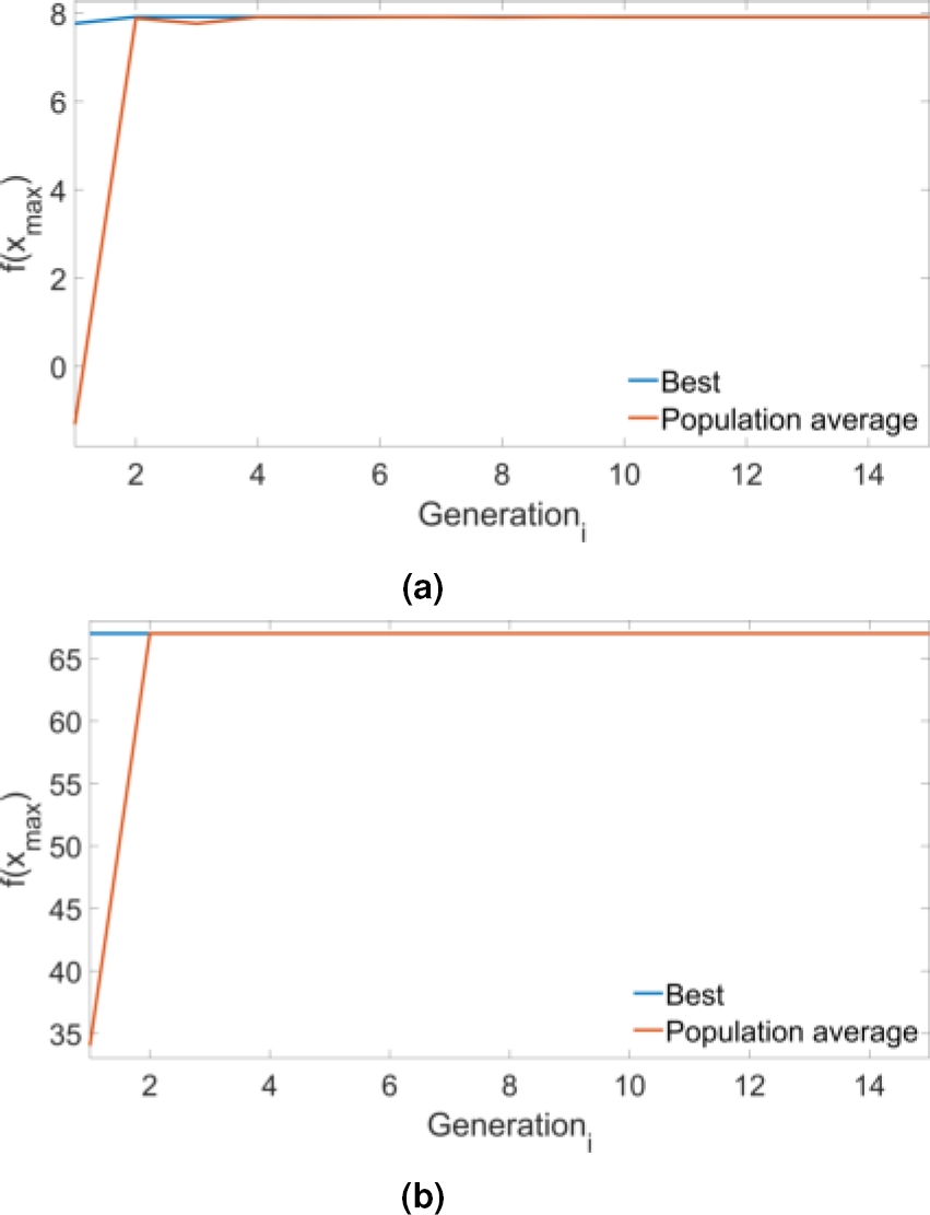
Fig. 2 Plot of the best and average values as a function of generation. The algorithm converged in the early generations. (a) Function f1 and (b) Function f2 with 15 generations on Harmony 

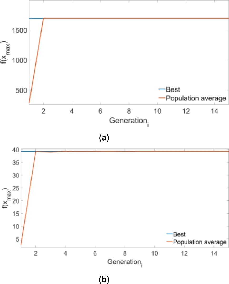
Fig. 3 Plot of the best and average values as a function of generation. The algorithm converged in the early generations. (a) Function f3 on Harmony and (b) Function f4 on Simulator SV1 with 15 generations, respectively 

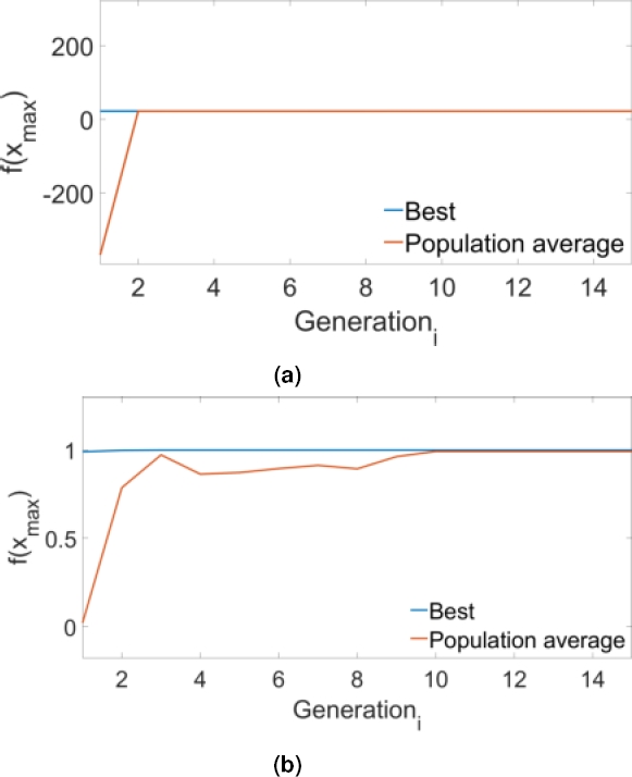
Fig. 4. of the best and average values as a function of generation. The algorithm converged in the early generations. (a) Function f₅ and (b) Function f₆ with 15 generations on simulator SV1 

They also have an average that describes how the function values near the optimum or even the optimum value have been found since early generations. This is a promising outcome, especially compared to simulation results from previous studies such as [²], [¹³] and [¹⁷] which predict favorable results.

4.2 Experiment 2: Python Implementation

In the second experiment, we ran ten generations per test for the Python implementation of the QGA, using 1,000 shots on f4 and f6 with the Aria-1 device, which contains 25 qubits. These limitations were set to stay within the budget. The number of executions was limited to three.

For the local simulator with the same characteristics mentioned in the previous experiment, we had 40 algorithm executions (runs). A comparison of the simulator run and the data obtained from the Aria-1 quantum device run is shown in Table 7.

In Table 7, we can see that the results on the quantum device are near the maximum, while the local simulator also shows greater accuracy in the other functions. The closest values are highlighted in bold.

4.3 Comparison of Local Simulator

Finally, we compare the two simulations made with the QGA versions. One simulation used the MATLAB ‘quantum’ package and the other used Amazon Braket in Python with our computing resources (Intel Core i7-9750 Processor (2.6 GHz) with 16 GB of RAM running Windows 11 Home with MATLAB 2023 and Python 3.11) to simulate quantum processing. Table 8 shows the mean, standard deviation, and median.

The MATLAB data shows a lower standard deviation compared to Python, as well as a good mean approximation toward the target. In Table 8, it is possible to observe that the median results closest to the maximum for Python are with f1 and f6, which also have a lower deviation. In the case of MATLAB, f1, f2, f4, f5, and f6 test functions show good performance, data that are shown in bold.

In Figure 5, the difference between the maximum value to be obtained, and the values generated by QGA on both platforms is shown where each function exhibits different behaviors. Additionally, the behavior with both libraries shows significant differences, which are consistent with Table 8. A high dispersion is observed for the case of Python (marked with a star).

Fig. 5 Differences between the best elements found and the maximum of all functions 

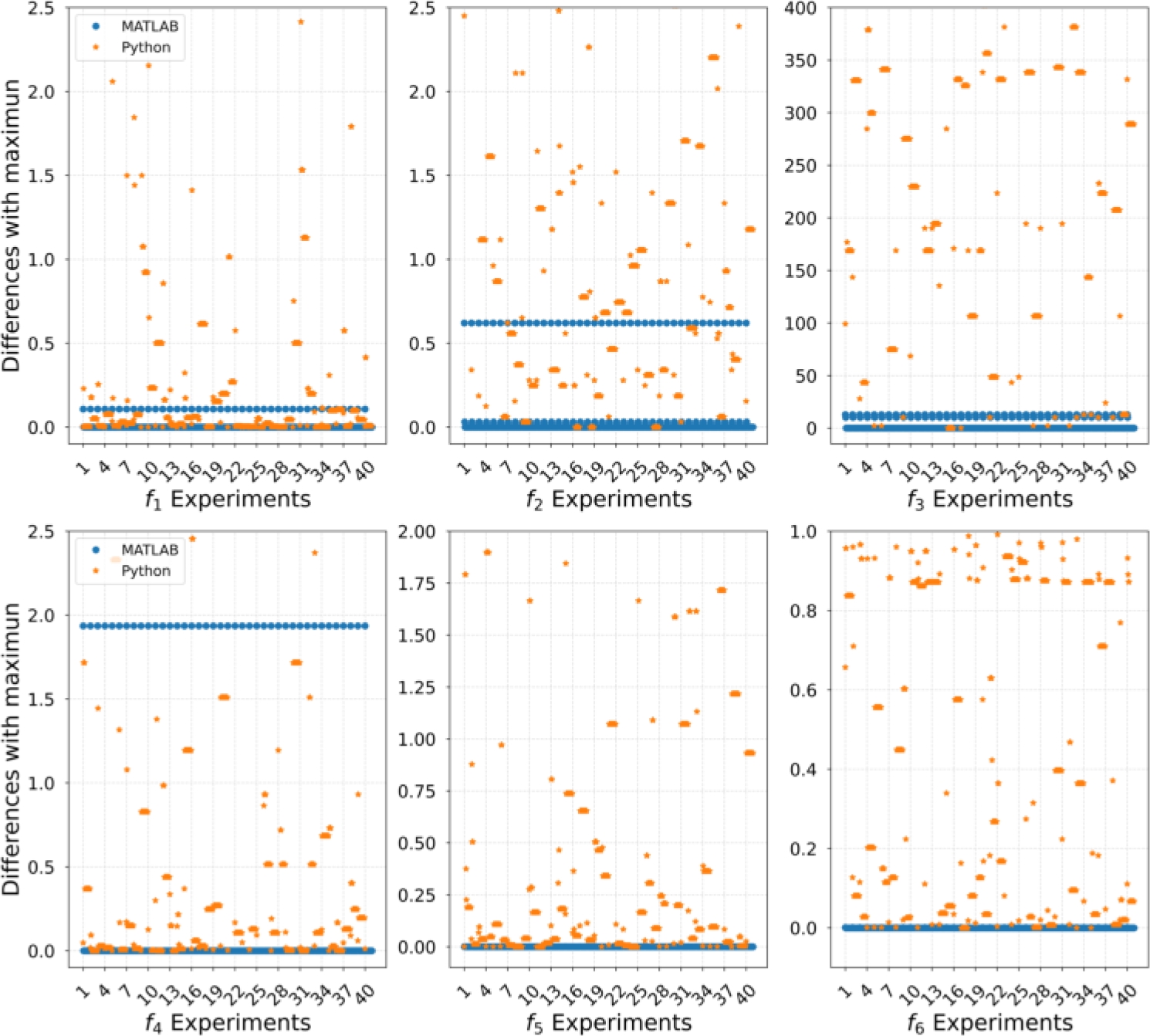
The observed wiggly points are due to the random nature of the algorithm in every run, where each execution begins with a new quantum population that evolves after each generation (15). With MATLAB, the jumps are more noticeable as it approaches the last generation of each run, containing better elements and resulting in almost zero difference.

In contrast, with Python, only some runs show improvement after each generation. For example, for test functions f1, f4, and f5, a behavior similar to that of MATLAB can be seen, but not for the other functions.

The distribution of the total of the best individuals obtained from the local simulator executions is shown in Figure 6 and Figure 7. Results obtained with Python are represented in green, while those obtained with MATLAB are in blue, with a dotted line indicating the maximum required value.

Fig. 6 Distribution of maximum findings for functions f1 - f3. Figures top MATLAB, bottom Python 

Fig. 7 Distribution of maximum findings for functions f4 - f6. Figures top MATLAB, bottom Python 

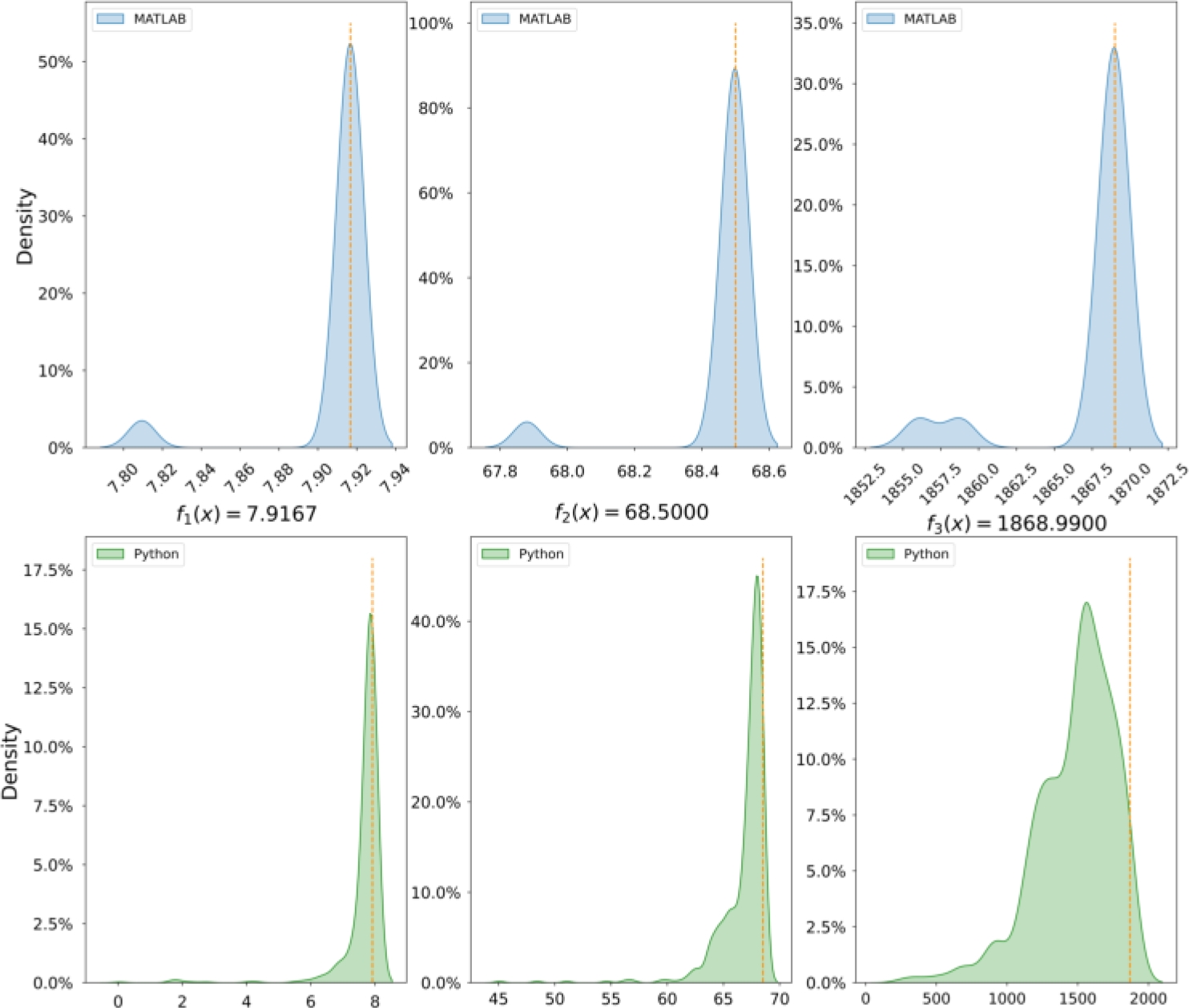
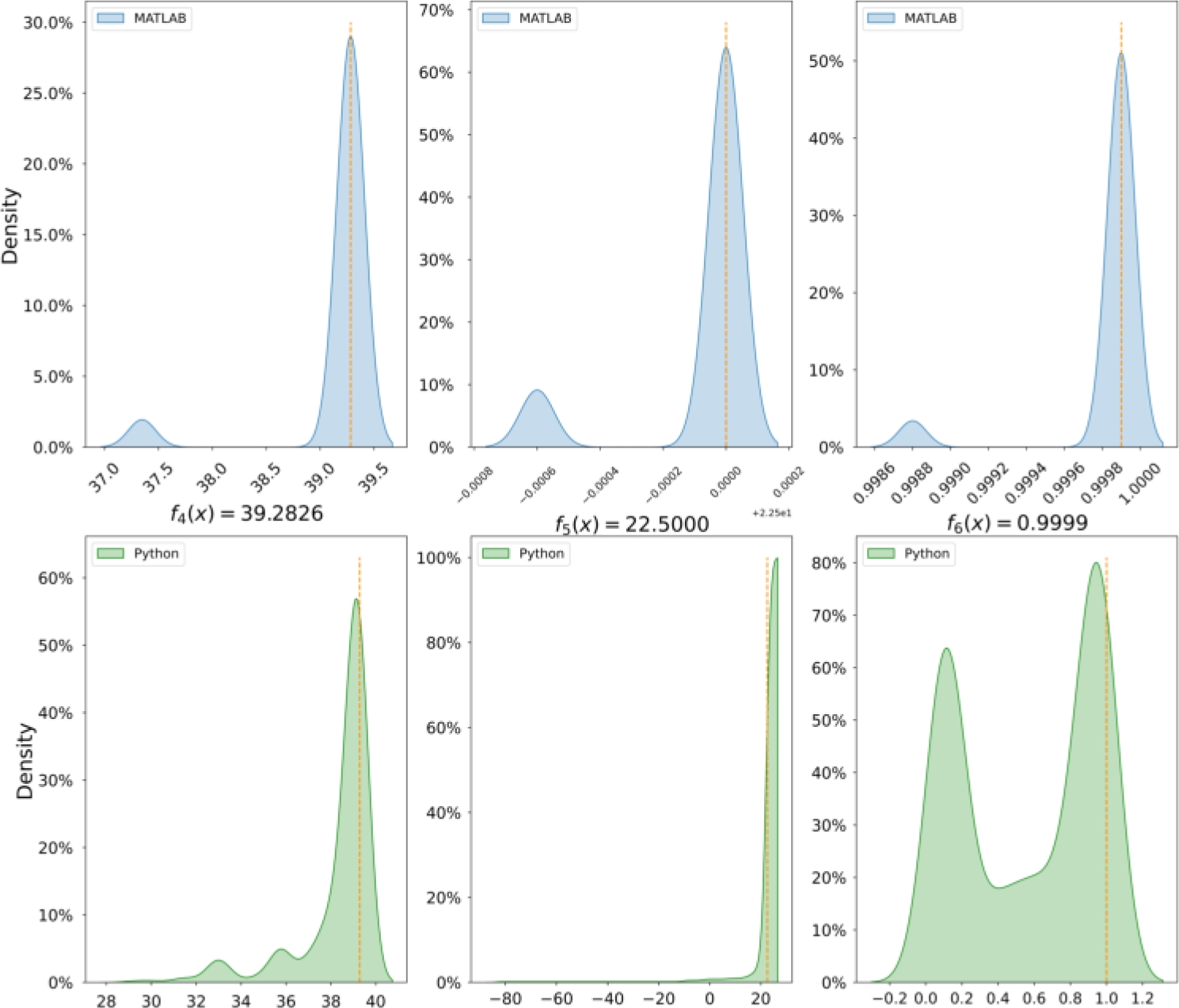
Both Figures (6 and 7) demonstrate the precision of MATLAB. Although Python and MATLAB both show that the highest percentage of the values obtained are close to the maximum required, it is evident that Python produces results that are further away from the maximum required value compared to MATLAB.

On the other hand, Table 9 shows the execution times with MATLAB using Harmony and with Python using Aria-1, as well as the times with the local simulator, available on both platforms. Additionally, Table 9 shows the particular time to generate the quantum population and the quantum mutation (quantum tasks), data obtained from the record that AWS makes on the Amazon Braket console.

Additionally, it is possible to observe a significant difference in the time described in Table 9. The average time results shown in Table 9 were obtained from approximately 583 quantum tasks with 100 shots in MATLAB. For Python results, approximately 534 tasks with 1,000 shots. It is imperative to provide additional information on operating hours to access specified quantum devices, such as Harmony and Aria-1.

These devices are available Monday through Friday from 12:00:00 to 03:00:00 UTC (Coordinated Universal Time). The above detail is significant since it introduces an additional waiting time to the total duration of the execution, a factor that is not considered in the current analysis because this time is independent of the chosen platform/programming language.

Likewise, AWS offers accessibility mechanisms such as Braket Direct, which facilitates time-bound requests for the use of specific quantum devices, and Hybrid Jobs, which encompasses hybrid quantum tasks.

The results shown in Figures 5, 6, and 7 depict the precision of the QGA in each test function. In that sense, statistics on the differences from the established maximum were obtained. A noticeable difference can be observed in test function f3 due to its multimodal behavior.

However, in general, we can see that for the rest of the test functions, the range of differences is much closer to the global maximum. The behavior of the QGA for the optimization of single-variable multimodal functions shows results consistent with previous studies, such as those by [¹³, ¹⁷, ¹⁸].

These studies conducted on simulators predict a good performance of the QGA. One of the significant advantages is the reduced number of generations or individuals required to find the maximum, resulting in substantial time and computational resource savings.

This performance is observed even in devices that, to date, contain a limited number of qubits. Two notable aspects of this work are time and cost, as access to a quantum device depends on the stable connection with AWS and the connection between AWS and the company owning the quantum computer.

Additionally, the queue of jobs waiting for each device and their established response times are crucial factors. These factors are important to consider when working with AWS, as the availability of various devices may be affected.

For example, when attempting to execute a task on certain devices, such as Aquila, the device may be suspended by the company, resulting in execution errors. Additionally, internet availability is another crucial factor to consider.