


 nueva página del texto (beta)
 Inglés (pdf)
 Artículo en XML
 Referencias del artículo
 Enviar artículo por email
 Citado por SciELO
  Similares en
SciELO
Similares en
SciELO 
 Permalink
1 Introduction
Cancer is a disease that is becoming more prevalent and is one of the main causes of death worldwide.
The GLOBOCAN 2018 database shows that 2018 saw 18.1 new million cases, with 9.6 million deaths. Lung cancer is the most diagnosed cancer. It has a mortality of 22% in men and 13.8% in women [6].
According to GLOBOCAN 2020 database, there were 19.3 million new cases and 10 million deaths in 2020. The mortality of lung cancer in men was 14.3%, and in women, it was 8.4% for the new cases that occurred in 2020 [31]. Radiologists specializing in medical radiology are the leading actors in detecting and diagnosing lung cancer.
Mastering the skills of a radiologist takes many years of practice; they are taught how to interpret images to diagnose and treat deseases by integrating extensive knowledge of clinical concepts [12]. Additionally, technological advances have allowed artificial intelligence techniques to be applied to detect these conditions [24, 16, 13].
In artificial intelligence, machine learning (ML) plays a leading role due to its high capacity for data processing. Machine learning is based on developing and training algorithms that can infer or predict a result based on a dataset.
Deep learning (DL) is a form of ML based on a multistage array of neural networks that learn from analyzing massive amounts of data. DL employs three main types of learning algorithms:
– Unsupervised learning, where data are not categorized, and the algorithm finds patterns that allow the data to be organized in some way;
– Semi-supervised learning, which uses partially labeled datasets;
– Supervised learning, which depends on the labels given to the training data.
DL includes several supervised learning techniques, such as recurrent neural networks (RNNs), convolutional neural networks (CNNs), and Deep Neural Networks (DNNs) [1]. Among the applications of CNNs, their extensive application in diagnosing medical images stands out.
The transfer learning (TL) technique applies a model pre-trained on millions of images from one domain to another domain with a smaller set of images. This technique favors the rapid development of models that provides the same performance results as the model trained with the massive dataset [15].
Some contributions from the scientific community concerning detecting cancer automatically using different classification algorithms are described below. Ramteke and Monali [26] propose an image classification method to classify images into two classes, normal and abnormal, based on the characteristics of the images and the automatic detection of abnormalities. The method consists of four main steps: a) preprocessing, b) feature extraction, c) classification, and d) post-processing. The K-nearest neighbor (KNN) algorithm is employed and is compared with a support vector machine (SVM) based image classifier. KNN achieves an accuracy of 80%, much better than the 69% accuracy obtained by the SVM.
Masood et al. [19] propose a computerized assistance system to support radiologists in lung cancer diagnosis based on DL using a dataset from the Medical Body Area Network (MBAN). This DFCNet model uses a fully convolutional neural network (FCNN), which is utilized to classify each detected spot in four stages of lung cancer. The effectiveness of the proposed work is assessed on different datasets with varying scanning conditions. Overall, the accuracies of CNN and DFCNet were 77.6% and 84.58%, respectively.
The experimental results illustrate the significance of the proposed method for detecting and classifying lung cancer nodules. Miah and Yousuf [20] present a lung cancer detection model using computed tomography (CT) images and image processing and neural networks. In this approach, the dataset is preprocessed using digital image recognition algorithms, the segmentation of areas of interest, and the classification of these segments using convolutional neural networks.
In the first step, a binary conversion technique detects cancer with a comparison value. In the second step, the image with cancer is segmented, and a feature extraction method is applied. These segments are used to train a neural network, and then, the system is tested with images with and without cancer. This system achieves an accuracy of 96.67%.
Sasikala et al. [28] utilize a CNN to categorize lung tumors as benign or malignant. This approach is based on taking regions of interest from the image; then, every slice is segmented to find tumors. The accuracy obtained with this method is 96%; it is more efficient than other traditional neural network methods.
The dataset is obtained from the Lung Image Database Consortium (LIDC) and the Image Database Resource Initiative (IDRI). Shaziya [30] proposes an automatic classification and detection system for lung cancer in medical images using DL. With a CNN model, the proposed method is meant to categorize spots on the lungs in pulmonary CT images from the LIDC dataset.
A total of 6,691 images containing nodules and non-nodules are provided as input to a four-layer 2D CNN model. The model is trained on 70% of the dataset, validated on 10% of the dataset, and tested on 20% of the dataset. The evaluation conducted on the test data resulted in an accuracy of 93.58%, a sensitivity of 95.61%, and a specificity of 90.14%.
On the other hand, the progress of information technology in the medical sector has required the development of communication protocols or standards for managing information in a simple, secure, and comprehensive manner. The most widely used protocol in the medical sector is DICOM. It addresses five general application areas:
Online image management.
Online image interpretation.
Online image printing.
Online image procedure management.
Offline storage media management.
This standard is a comprehensive specification of the elements necessary to achieve a practical level of automatic interoperability among biomedical imaging systems. DICOM provides detailed engineering information that can be used in interface specifications to enable connectivity between various pieces of vendor equipment.
The standard describes how to format and exchange the associated medical image information within and outside the hospital (e.g., teleradiology and telemedicine, among others) [5]. Among the research works that have utilized the DICOM standard is that of Angarita et al. [2], in which the MÉDICO MWEB system is described.
This system was developed with a data structure based on the DICOM standard model, tools (enhancement tools, measurements tools, filters) for visualization and analysis, an intuitive exploration and navigation system for image collection accessible via the web with any browser, and other added features.
A three-layer architecture, a design that introduces an intermediate layer into the process, was used for project development. In this type of architecture, each level is given a simple task, allowing the design of scalable architectures, i.e., they can be easily expanded if the requirements change.
Through the application, DICOM files can be uploaded to the public or private directory of the user, and it also manages an interface for managing the fields of the file; fields can be added, modified, and deleted.
Similarly, DICOM files can be created from JPG images, registering basic standard data that will be attached to the image in the DICOM file. All processes are handled through the JDT library and with an interface developed in JSP and Ajax.
Archie and Marcus [3] describe the DICOM browser application as a software system that views and modifies DICOM file information. Its installation requires the user to have computer knowledge beyond primary computer usage. This application is part of the XNAT software system, defined as an open-source application available for generic use in medical applications.
Similarly, installing XNAT requires advanced computer usage knowledge. XNAT presents a series of steps for installing a pre-trained deep learning model. Doing this requires the user to learn hardware techniques (NVIDIA) and advanced configurations.
Castro et al. [8] present a DICOM image viewer based on a hybrid architecture that uses client-server, model-view-view-model (MVVM), and N-layer architectural patterns. The client-server style defines a relationship between two applications in which one sends requests to another for processing.
The fundamental concept of MVVM is to separate the model from the view by introducing an abstract layer that allows more accessible and more scalable management of interaction and states. For the development of the client-server application, the HTML5 and JavaScript libraries were used on the client side, and C# with .NET Framework version 4 was used on the server side. Other JavaScript libraries that were used include WADO and KnockoutJS.
Vellez et al. [33] describe Visilab Viewer as a web application that adheres to the DICOM standard. It uses a Flask REST API architecture, Waitress as a WSGI server, and PyTorch as a library for deduction using DL techniques due to its widespread use in both research and commercial applications and because of the ability to import models from other systems.
For CNNs to make deductions, it is necessary to obtain image segments that fit an image with a specific magnification and divide them into patches of the size requested by the CNN. Finally, inference will be achieved by applying a diagnostic rule. Vellez et al. developed a server that manages the Difference in Proportions of Labels (DPL) module using Python 3 and Flask, as it natively allows multiple requests to be responded to simultaneously.
Thus, the system can have numerous users simultaneously or receive different inquiries from the same user. This system uses a database with breast cancer images and three different models, which are HER2 classification, the Ki67 proliferation index, and tumor area detection in H&E WSI using the following neural networks: AlexNet (AN), GoogLeNet (GN), VGG-16 (VGG), ResNet-101 (RN), and DenseNet-201 (DN).
Pham et al. [23] present the VinDr system, which has two branches related to the classification of CT images of the chest VinDr-ChestCT and XR images of the chest VinDr-ChestXR. This system focuses on identifying various parts of the body; it is a DL classifier that takes an unknown X-ray as an input image and classifies it into one of five groups, including abdominal X-rays, adult chest X-rays, pediatric chest X-rays, spine X-rays, and others.
From a functional standpoint, a reliable DICOM image router must ensure two essential requirements, including (1) an approximately 100% classification accuracy and (2) providing fast inference.
Mathematically, this supervised multiclass classification task assigns a class label to each input sample. In the present work, a method is proposed to assist the radiologist in decision-making concerning the diagnosis of lung medical images.
This method consists of an architecture that integrates a) deep learning models, b) custom private DICOM tags, and c) a viewer for displaying classification results. This paper is organized as follows. Section 2 presents the basic theory of this research. Section 3 describes the proposed architecture. Section 4 presents the experiments conducted. Lastly, Section 5 presents the conclusions and future work.
2 Background
In this section, the related concepts for this research are presented. Section 2.1 describes the DICOM standard. Section 2.2 introduces the concept of “anonymization” which relates to security and confidentiality for the patient, the radiologist, and all personnel involved in the review and classification of medical images.
Section 2.3 describes the architecture of the convolutional neural networks used in deep learning. Section 2.4 describes transfer learning. Section 2.5 discusses the Machine Learning .NET library (ML.NET). Section 2.6 discusses deep learning models in ML.NET. Lastly, Section 2.7 discusses evaluation metrics for machine learning models.
2.1 The DICOM Standard
DICOMfn is a crucial concept in the world of digital imaging. The absence of a standard inhibits usability and the exchange of images, forcing users to deal with many data formats and convert data from one format to another.
Any image file, in addition to pixel data, contains metadata. Metadata describes the image and plays a significant role in digital imaging. While in general-purpose image formats, metadata may be limited to describing the pixel array, in formats for medical applications, they can describe the image, instrument configuration, image acquisition parameters, and any other elements of interest related to the imaging workflow. The standard helps define the metadata section for the correct use and interpretation of the image.
In the early 1980s, an association of users and healthcare professionals, the American College of Radiology (ACR), and the National Electrical Manufacturers Association (NEMA) began defining a new standard for encoding and exchanging digital medical images. In 1993, the ACR-NEMA committee presented DICOM as a standard with more functionality and long-term vision than previous standardization attempts [18].
Since then, DICOM has been strengthened by including and collaborating with other standards, such as the European Committee for Standardization (CEN) and ISO TC 215 Health Informatics. Figure 1 presents the general communication model for the storage of medical information on any removable media [21].
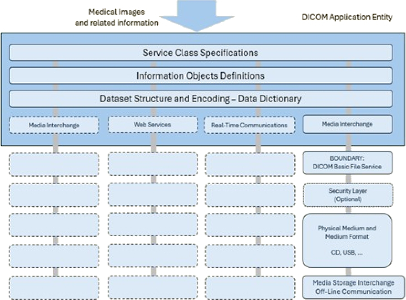
Applications can use any of the following transport mechanisms: The DICOM message and upper-layer service provides independence from specific physical network support and communication protocols such as TCP/IP.
The DICOM web service API and HTTP service allow the use of common hypertext and the associated protocols for transporting DICOM services. The basic DICOM file service provides access to storage media regardless of specific media storage formats and file structures.
Real-time DICOM communication provides the real-time transport of SMPTE and RTP-based DICOM metadata. The current version of the DICOM standard is composed of the following 22 partsfn:
– PS3.1 Introduction and overview.
– PS3.2 Conformance.
– PS3.3 Information object definitions.
– PS3.4 Service class specifications.
– PS3.5 Data structures and encoding.
– PS3.6 Data dictionary.
– PS3.7 Message exchange.
– PS3.8 Network communication support for message exchange.
– PS3.9 Retired.
– PS3.10 Media storage and file format for media interchange.
– PS3.11 Media storage application profiles.
– PS3.12 Formats and physical media.
– PS3.13 Retired.
– PS3.14 Grayscale standard display function.
– PS3.15 Security and system management profiles.
– PS3.16 Content mapping resource.
– PS3.17 Explanatory information.
– PS3.18 Web services.
– PS3.19 Application hosting.
– PS3.20 Imaging reports using HL7 clinical document architecture.
– PS3.21 Transformations between DICOM and other representations.
– PS3.22 Real-time communication (DICOM-RTV).
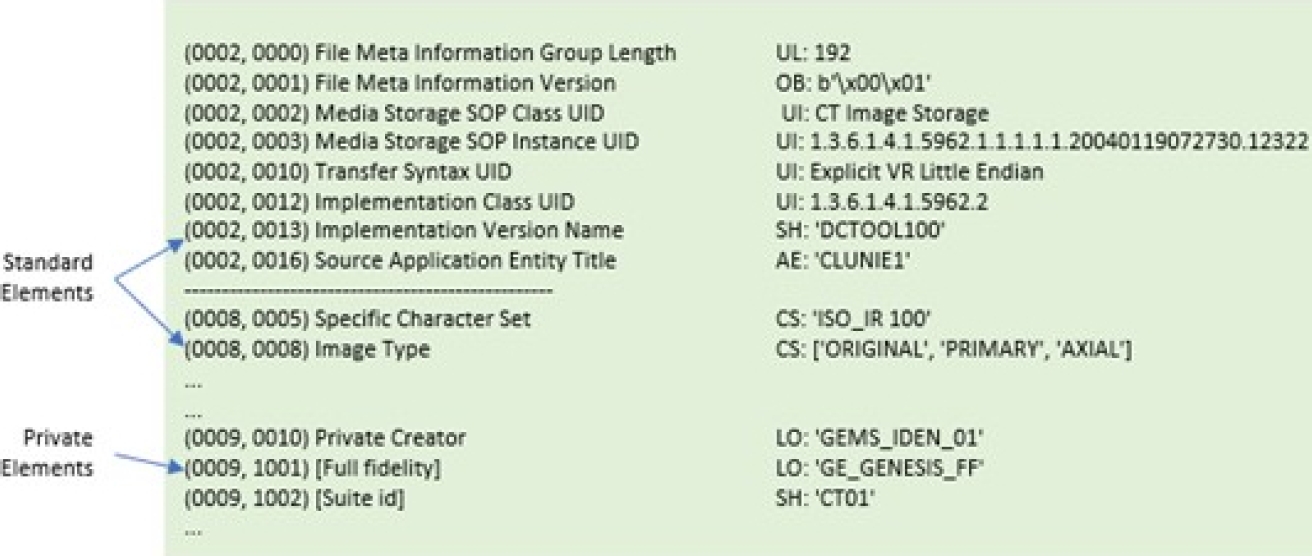
This research focuses on Part 5, Data Structures and Encoding, for accessing standard and private data elements. A data element tag uniquely identifies a data element. Data elements in a dataset shall be ordered by increasing the data element tag number and shall appear at most once in a dataset.
Two types of data elements are defined: 1) standard data elements have an even group number that is not 0000, 0002, 0004, or 0006, and 2) private data elements have an odd group number that is not 0001, 0003, 0005, 0007, or FFFF. The DICOM standard allows the use of standard and private elements as long as they are not already in use.
The reserved elements, both standard and private, are those mentioned above. Figure 2 depicts the structure of two standard data elements, with the group field having even values of 0002 and 0008, and a standard private data element, with the group field having an odd value of 0009.
2.2 DICOM Anonymization
DICOM emphasizes the security and protection of the information of the radiologist, patient, and all equipment related to the review and classification of medical images. DICOM establishes in part PS3.15fn the elements and actions to be executed when anonymizing pertinent information—Table E.1-1a. De-identification Action Codes state the actions on these elements in Table E.1-1.
Application-Level Confidentiality Profile Attributes define the elements and attributes for this purpose. Our proposal adheres to this directive, and to do this, it automatically executes this process when accessing any file with this format. Anonymization consists of removing or replacing all tags specified in Table E.1-1.
Our proposal does not request or store the personal information of any patient, radiologist, doctor, or anyone related to this type of medical activity. If, for any reason, the provided DICOM file contains any of the tags listed in this table, the value of each of these is replaced with a string of the form “**.**”; this indicates that there was a previous value that was replaced by this string.
This string is used only for demonstrative purposes. The application fulfills the directions in Table E.1-1a. None of these tags are removed from the original file. If this framework application updates any of these tags, a new file is generated by adding the following name ending:
“-Anonymous”, between the original name and its extension type. Figure 3 displays an original DICOM file with some patient information in it. Figure 4 shows the result from this framework, which shows that confidential patient information was replaced with the dummy string “**.**”.
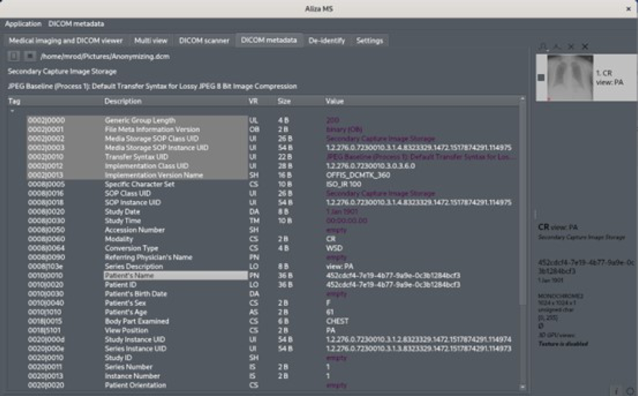
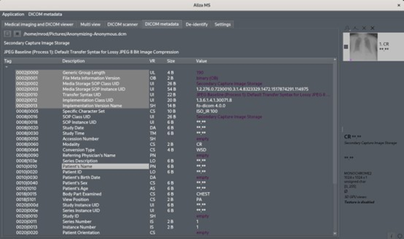
Fig. 4 File from Figure 3 with patient-identifying data (patient’s name) replaced with “**.**” string
2.3 Deep Learning
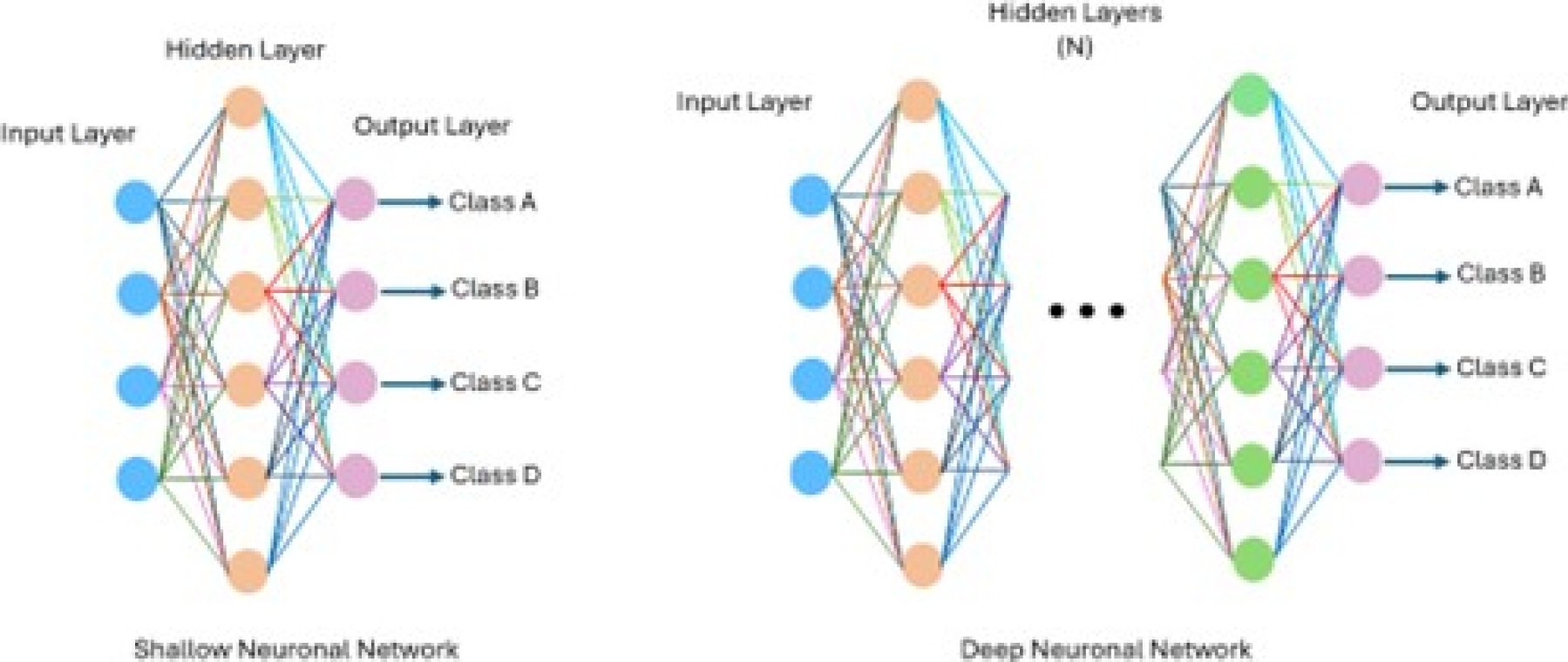
Deep learning, a branch of ML and AI, is regarded today as a core component of the current Fourth Industrial Revolution (4IR or Industry 4.0). DL technology originated from artificial neural networks (ANN), and due to its ability to process and learn from data, it has become a significant topic in computer science; it has been widely applied in various areas such as healthcare, visual recognition, text analysis, and cybersecurity. However, building a reasonable DL model is difficult due to the constantly changing nature and variations in real-world problems and data. Sarker et al. [27] illustrate the difference between a shallow neural network (SNN) and a DNN, where an SNN has only one layer. The DNN consists of multiple layers, as shown in Figure 5. Similarly, Sarker et al. [27] define the following categories of DL:
Supervised: Uses labeled training data.
Unsupervised: Utilize unlabeled datasets.
Semi-supervised: Combines both supervised and unsupervised.
Reinforcement: Approach focused on the context of the considered problem.
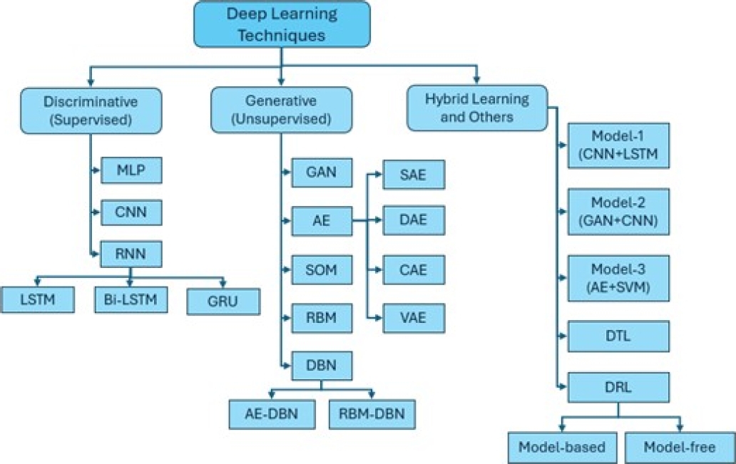
Deep learning is divided into the following three branches:
DNN with supervised/discriminative learning.
DNN with unsupervised/generative learning.
Hybrid learning combining the above models, as shown in Figure 6.
CNNs are based on multi-layer neural networks that can identify, recognize, and classify objects and detect and segment objects in images. The CNN is a well-known architecture of discriminative DL that can learn straight from the input object without requiring human involvement for feature extraction. Figure 7 shows the basic structure of a CNN [32]. A convolutional neural network consists of a convolutional layer, poling, an activation function, and a fully connected layer.

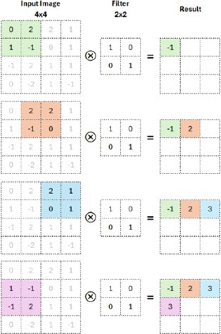
– Convolutional layer: This step applies filters to the input data (input image). The kernel is a set of integer values. The CNN filter weights are a set of randomly chosen integers. The kernel learns to extract significant features because these weights are modified during training. It calculates the inner product of the images of all data pairs in the feature space. This mechanism is shown in Figure 8.
-
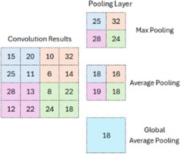
– Pooling: This is used to reduce the size of the feature map once the filter has been applied. Down-sampling is an essential part of pooling, which helps decrease the upper layers’ complexity. The number of filters is not affected by it. The max pooling method is one of the most used methods.
The image is divided into rectangular subregions, and the maximum value within each subregion is selected. A standard max pooling size is 2 × 2. As shown in Figure 9, when pooling is applied in the upper-left corner, the operation shifts to the upper-right corner and moves by two steps. The filter moves in 2×2 steps to perform pooling.
-
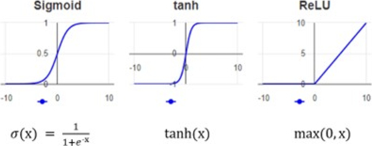
– Activation function: The non-linearity layer allows the generated output to be changed. This layer is used to limit or oversaturate the output. Each activation function in a neural network fulfills the essential process of mapping the input to the output.
The input value is calculated as the weighted sum of the neuron’s input and its bias. This bias implies that the activation function decides whether a neuron is activated in response to a given input, generating the corresponding output. Figure 10 shows the most common activation functions.
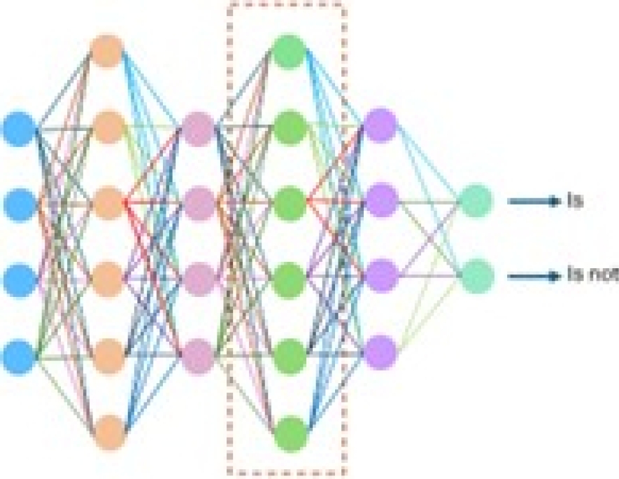
– Fully connected layer: This step arranges neurons in groups. As shown in Figure 11, every node in every layer is connected directly to another node in the previous layer and next layer.
2.4 Transfer Learning
DL has two types of TL: feature extraction and fine-tuning. A dataset like ImageNet is used for feature extraction, but the top layer used for classification purposes will be removed. In addition to the pre-trained model, a new classifier is trained to complete the classification task.
The pre-trained model is considered an arbitrary feature extractor that extracts valuable features from the new dataset. For fine-tuning, the weights of the pre-trained model are taken as the initial values for the latest training and are reworked and fine-tuned in the process.
In this case, the weights are adjusted from generic feature maps to specific attributes related to the new dataset. Fine-tuning aims to adapt the generic features to a particular task instead of overriding generic learning [29]. The work [25] describes how Resnet50V2 was trained using the ImageNet dataset. Databases from different sources are used to retrain existing models like the ones mentioned here. One of these sources is Kaggle, where there are datasets with CT medical images of various types of cancer. Additionally, there are open-source libraries such as Microsoft’s Machine Learning .NET (ML.Net) library, which provides support for applying transfer learning from an application developer’s standpoint.
2.5 Machine Learning .NET Library
ML.NET is a cross-platform library tool designed to build and train ML models within .NET applications. ML.NET aims to provide the same capabilities data scientists and developers can find in the Python ecosystem. ML.NET is based on the classic ML operation concept: gather data, configure the algorithm, train, and deploy.
ML.NET allows the use of deep learning models such as TensorFlow and Open Neural Network Exchange (ONNX), enabling developers to train CNN classification models. The entire ML.NET library is built on the .NET Core framework [11].
2.6 Deep Learning Models with ML.NET
Below are descriptions of the deep learning models InceptionV3, MobileNetV2, ResNetV2101, and ResNetV250:
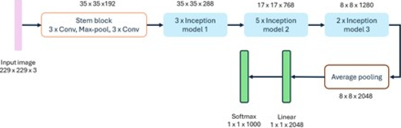
– InceptionV3: The InceptionV3 model [7] utilizes convolutional filters of different sizes, allowing it to obtain receptive fields of other areas. To reduce the design space of the network, it embraces a modular system followed by a final union, thus completing the fusion of features from different scales. This model considers typical congestion and performance problems; better results can be obtained using asymmetric kernels and bottlenecks and by replacing large filters with smaller ones [9]. The configuration of the InceptionV3 model is shown in Figure 12.
-
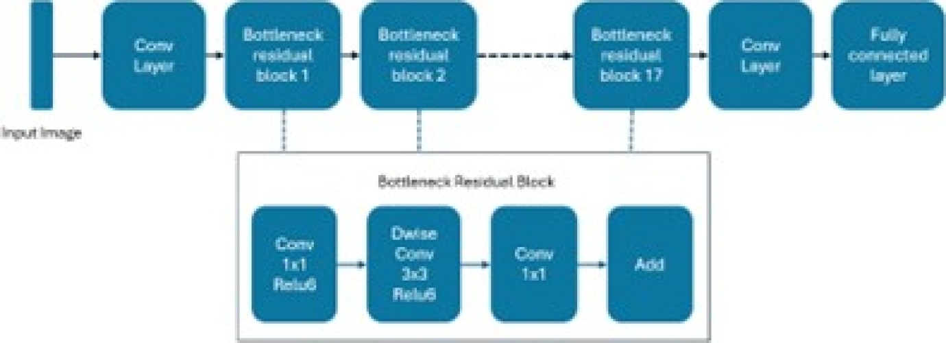
– MobileNetV2: This model targets portable devices. It is distinct from other CNN architectures, where its links are between bottleneck layers. The middle layer expansion also employs deep levels to filter out non-linear attributes. The MobileNetV2 platform includes 32 convolution layers followed by 19 bottleneck layers. For small datasets, it is not easy to train, and the image classification task becomes challenging.
This model mitigates this effect by preventing overfitting, and it is a fast and successful architecture that optimizes memory consumption with a low error margin. Additionally, the design of MobileNetV2 provides fast transaction execution during experimentation and optimization of parameters [17]. This model is depicted in Figure 13.
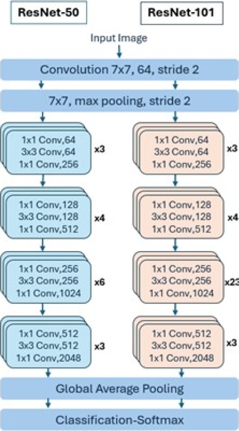
– ResNetV2101 and ResNetV250: The Microsoft research team developed ResNet to ease the difficulty of training deeper neural networks. The main idea of ResNet is to learn the additive residual function using shortcut equivalence mappings. It has versions with 18, 34, 50, 101, and 152 weight layers. Instead of learning non-discriminative functions, it utilizes residual functions by adopting skip connections. Unlike VGG, ResNet uses shortcut connections in feedforward neural networks. Figure 14 depicts the layers of these models [4].
2.7 Evaluation Metrics for ML Models
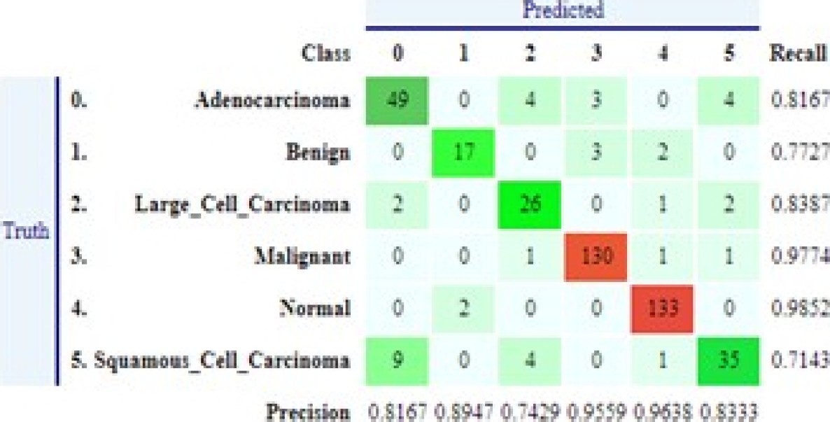
Below, we describe the concepts and metrics used to assess the performance of machine learning models. Most metrics use relevant information from the confusion matrix about the algorithm and classification rules. This matrix registers the differences between the actual (rows) and predicted (columns) classifications [14] , as shown in Figure 15. The following metrics are calculated using values from the confusion.
Precision: It is the fraction of true positive (TP) parts divided by the total number of units predicted positively (column sum of predicted positives).
True positives are the parts that have been labeled as positive by the model and are positive. False positives (FP) are the parts labeled as positive by the model that are actually negative [14]:
Recall: This is the fraction of true positives divided by the total number of positive elements (sum of rows of true positives). Specifically, false negatives (FN) are the elements labeled as false by the model that are actually positive [14]:
Accuracy: The sum of true positives (TP) and true negatives (TN) in the numerator is divided by all entries in the confusion matrix. TP and TN, found on the main diagonal, represent correctly classified instances. Accuracy reflects the probability that the model’s prediction is correct [14]:
F1-score (binary case): It is the weighted average between precision and recall, where the best value of the F1-score is one and its worst value is zero. The contribution of precision and recall are the same int the F1-score, and the harmonic mean helps find the best proportion between the two quantities [14]. The F1-score will detect any weaknesses in the prediction algorithm if any such weaknesses exist:
F1-score (multiclass case): For multiclass cases, the F1-score involves all classes. To achieve this, we need a multiclass measure of precision and recall to be inserted into the harmonic mean. These metrics can have two distinct specifications, resulting in two other metrics: the micro F1-score and macro F1-score.
For the calculation of the macro and micro F1-score, the precision and recall are now needed for all classes. Formulas (5) and (6) illustrate the calculation of precision and recall for a generic class k [14]:
Macro F1-score: The macro average precision and macro average recall are needed to calculate this parameter. Formulas (7) and (8) describe these metrics; they are calculated as the arithmetic mean of the metrics for individual classes.
Formula (9) presents the macro F1-score function. Macro Average precision (MAP), Macro Average recall (MAR) and MacroF1-score (MF1-score) are defined as:
Micro F1-score: To obtain the micro F1-score, micro-average precision, and micro-average recall should be calculated first. It considers all units together without regard to possible class differences.
These metrics are calculated as follows: It is observed that equations (10) and (11) have the same values; therefore, the average F1 precision is calculated in the same way [14]. Micro Average precision(uAP) and Micro Average recall are defined as:
LogLoss: This represents the average logarithmic loss of the classifier. It measures the performance of a classifier based on how much the predicted probabilities diverge from the true class label. A lower value indicates a better model. A perfect model, which predicts a probability of one for the true class, will have a logarithmic loss of zero.
Macro-accuracy: It represents the average macro precision of the model. The precision of each class is calculated, and the macro precision is the average of these precisions (macro-average = macro-F1-score).
Micro-accuracy: It represents the average micro precision of the model (micro-average).
3 Proposed Architecture
In this section, the proposed architecture for integrating different CNNs with the custom tags introduced in the DICOM communication standard to support decision-making in lung cancer diagnosis is presented. Two public Kaggle databases containing CT images were used to train the CNN algorithms. The predictions of the algorithms are stored in custom DICOM tags. Section 3.1 presents the proposed architecture. Section 3.2 describes the dataset. Section 3.3 outlines the implementation of DICOM private tags.
Section 3.4 describes the implementation of deep learning models. Lastly, Section 3.5 discusses the interaction between learning models and DICOM.
3.1 Description of the Proposed Architecture
The blocks composing our proposal are shown in Figure 16. Three main blocks interact with each other to provide recommendations to the radiologist. The Deep Learning Models block trains the model using the desired algorithm and makes predictions based on the provided image. The DICOM Parser/Updater block facilitates access to the input file to be predicted. It can be a simple image in the JPEG or PNG format or a file containing the entire DICOM standard dataset in addition to the image. This framework does not constrain the file type, size, quality, or consistency.
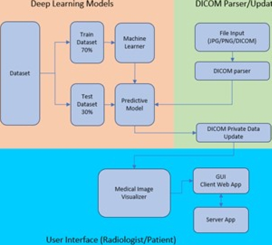
The User Interface (radiologist/patient) block allows the raiologist or patient to interact with the complete application. It is worth mentioning that the training and prediction tasks are performed on the server where the application runs, while the tasks of displaying results, selecting a DICOM file or image, and executing instructions are performed from the client application. The application code is available at GitHubfn.
3.2 Dataset Description
Two different datasets were obtained from the public Kaggle repository: CTfn Scan Images of Lung Cancer and IQ-OTHNCCDfn Lung Cancer Dataset. These datasets contain CT medical images of various types of cancer and of healthy individuals. The images are labeled based on the type of disease.
Table 1 shows the original class names of the CT Scan Images of Lung Cancer dataset and the names and index assigned for this research. Table 2 shows the names and index assigned to the IQ-OTHNCCD Lung Cancer dataset that will be used in the remainder of the paper.
Table 1 CT scan images of lung cancer dataset class names and indexes
| Name | Index | Assigned Name |
| Adenocarcinoma_left.lower. lobe_T2_N0_M0_Ib | 0 | Adenocarcinoma |
| Benign | 1 | Benign |
| Large.cell.carcinoma_left.hilum_T2_N2_M0_IIIa | 2 | Large_Cell_Carcinoma |
| Malignant | 3 | Malignant |
| Normal | 4 | Normal |
| Squamous.Cell.squamous.cell.carcinoma_left. hilum_T1_N2_M0_IIIa | 5 | Squamous_Cell_Carcinoma |
3.3 Implementation of DICOM Private Tags
DICOM private tags are elements that do not have any meaning or encoding in the standard. This self-registration scheme allows each developer to define their own set of private data, the meaning of which must be published in the provider’s DICOM documentation.
Developers can document essential values in a structured way in these private elements [10]. The DICOM standard defines private elements and establishes an effective way to use them. These private elements contain information not in standard data elements, such as manufacturer-specific information [22].
In our proposal, the DICOM standard was applied to use these private tags to store the prediction of each pre-trained model in a different private data element. The tag x0055 was defined as a private element for registering the prediction results of the trained models.
It is worth mentioning that the framework verifies whether this tag is in use; if it is, a new one is calculated by incrementing by two until another tag is available. Table 3 shows the element x0055, 0010 added to the DICOM private elements.
Table 3 DICOM private element x0055, 0010
| Private Tag | Description | Data |
| x0055,0010 | Private Creator | UACJ_VISOR |
| x0055,1010 | Model | InceptionV3.zip |
| x0055,1011 | Dataset | IQ-OTHNCCD Lung Cancer Dataset |
| x0055,1012 | Date | 2024 04 21 09:23:52.123 |
| x0055,1013 | FileName | 000160.png |
| x0055,1014 | FileSize | 89.364kB |
| x0055,1015 | Class | Prediction(%) |
| x0055,1016 | Malignant | 99.01 |
| x0055,1017 | Benign | 0.99 |
| x0055,1018 | Normal | 0 |
| x0055,1019 | Model | MobilenetV2.zip |
| x0055,101a | Dataset | IQ-OTHNCCD Lung Cancer Dataset |
| x0055,101b | Date | 2024 04 21 09:23:52.665 |
| x0055,101c | FileName | 000160.png |
| x0055,101d | FileSize | 89.364kB |
| x0055,101e | Class | Prediction(%) |
| x0055,101f | Malignant | 100 |
| x0055,1020 | Benign | 0 |
| x0055,1021 | Normal | 0 |
| x0055,1022 | Model | ResnetV2101.zip |
| x0055,1023 | Dataset | IQ-OTHNCCD Lung Cancer Dataset |
| x0055,1024 | Date | 2024 04 21 09:23:56.053 |
| x0055,1025 | FileName | 000160.png |
| x0055,1026 | FileSize | 89.364kB |
| x0055,1027 | Class | Prediction(%) |
| x0055,1028 | Malignant | 99.98 |
| x0055,1029 | Benign | 0.02 |
| x0055,102a | Normal | 0 |
| x0055,102b | Model | ResnetV250.zip |
| x0055,102c | Dataset | IQ-OTHNCCD Lung Cancer Dataset |
| x0055,102d | Date | 2024 04 21 09:23:57.912 |
| x0055,102e | FileName | 000160.png |
| x0055,102f | FileSize | 89.364kB |
| x0055,1030 | Class | Prediction(%) |
| x0055,1031 | Malignant | 99.99 |
| x0055,1032 | Normal | 0 |
| x0055,1033 | Benign | 0 |
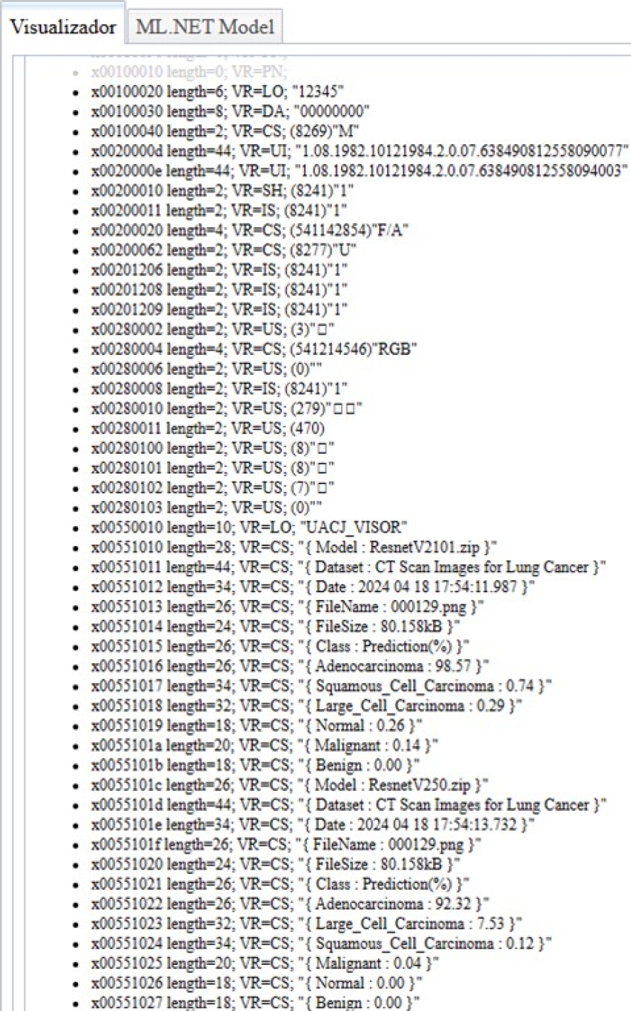
These added custom tags are used to show the percentage probability of each class, predicted by each deep-learning model. This information is shown for each model in the implemented viewer.
In Table 3, the tag x0055, 0010 is a private element with the value UACJ_VISOR, which reserves a block of ele-ments. The element x0055, 1010 is part of this block; the “10” in the label of element x0055, 10xx corresponds to the “10” in the label of the private element x0055, 0010.
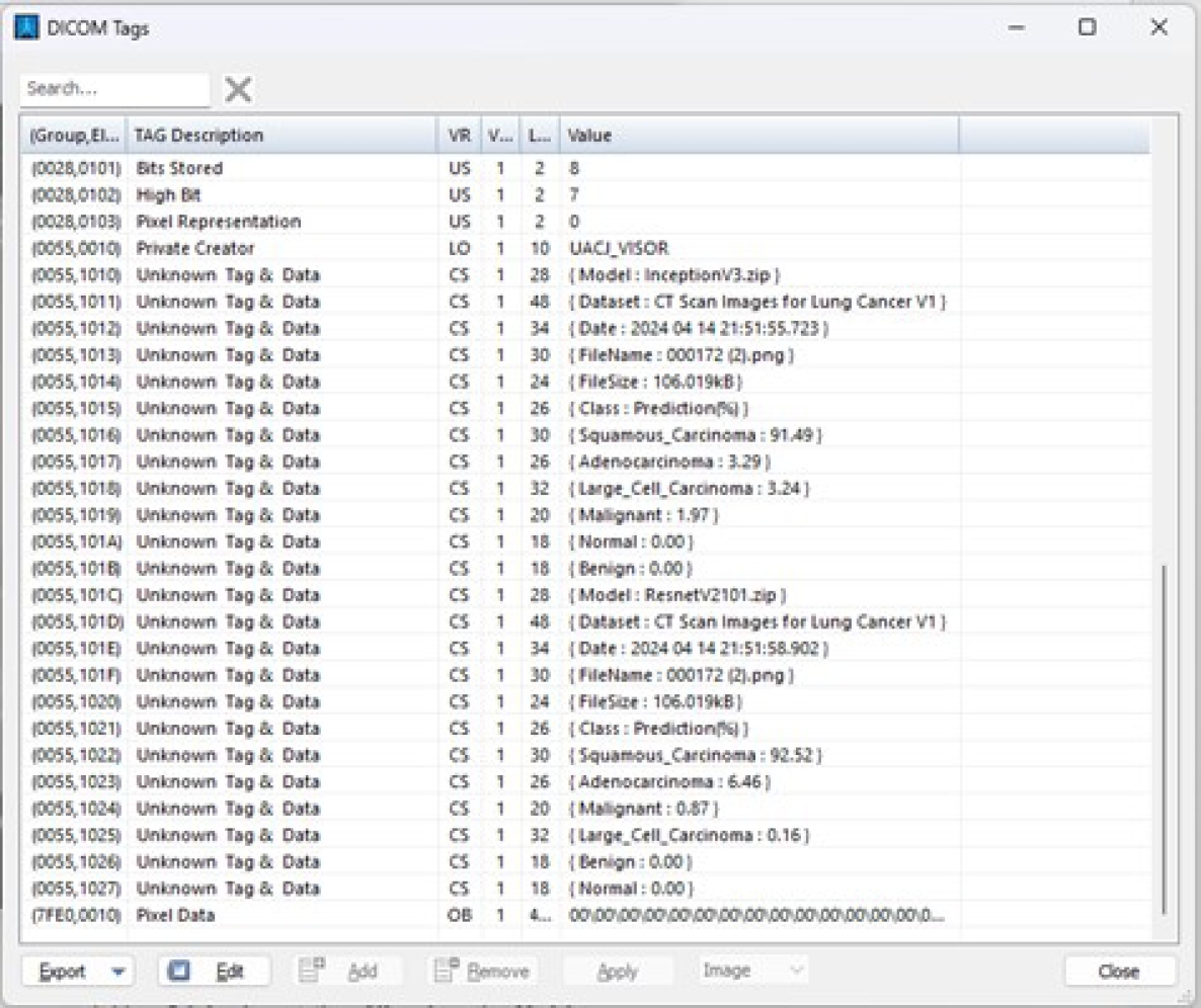
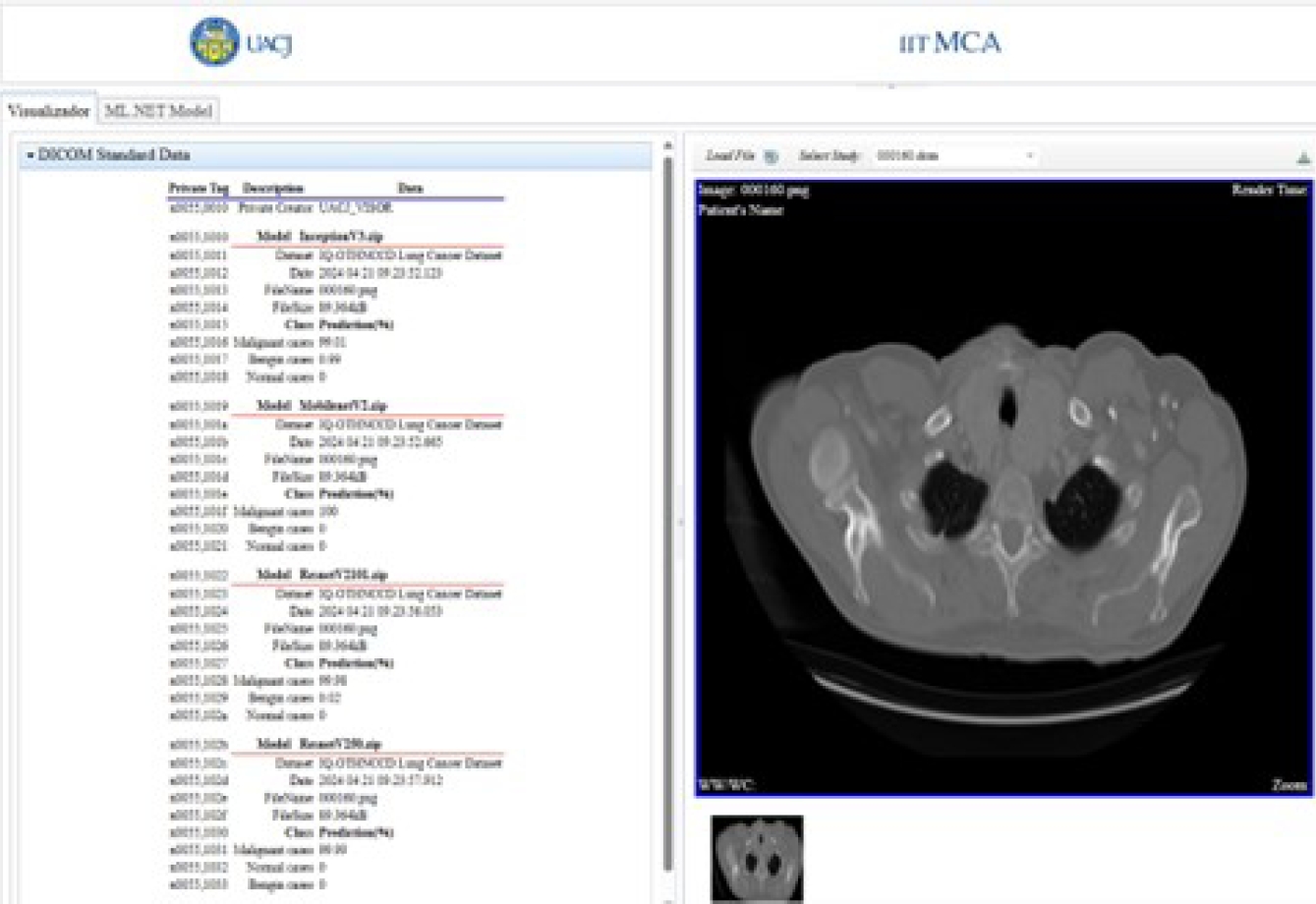
The predicted results and model are stored starting from private element x0055, 1010. Once the predicted results are stored in these private tags, they are displayed in the viewer’s DICOM tag panel, as shown in Figure 17.
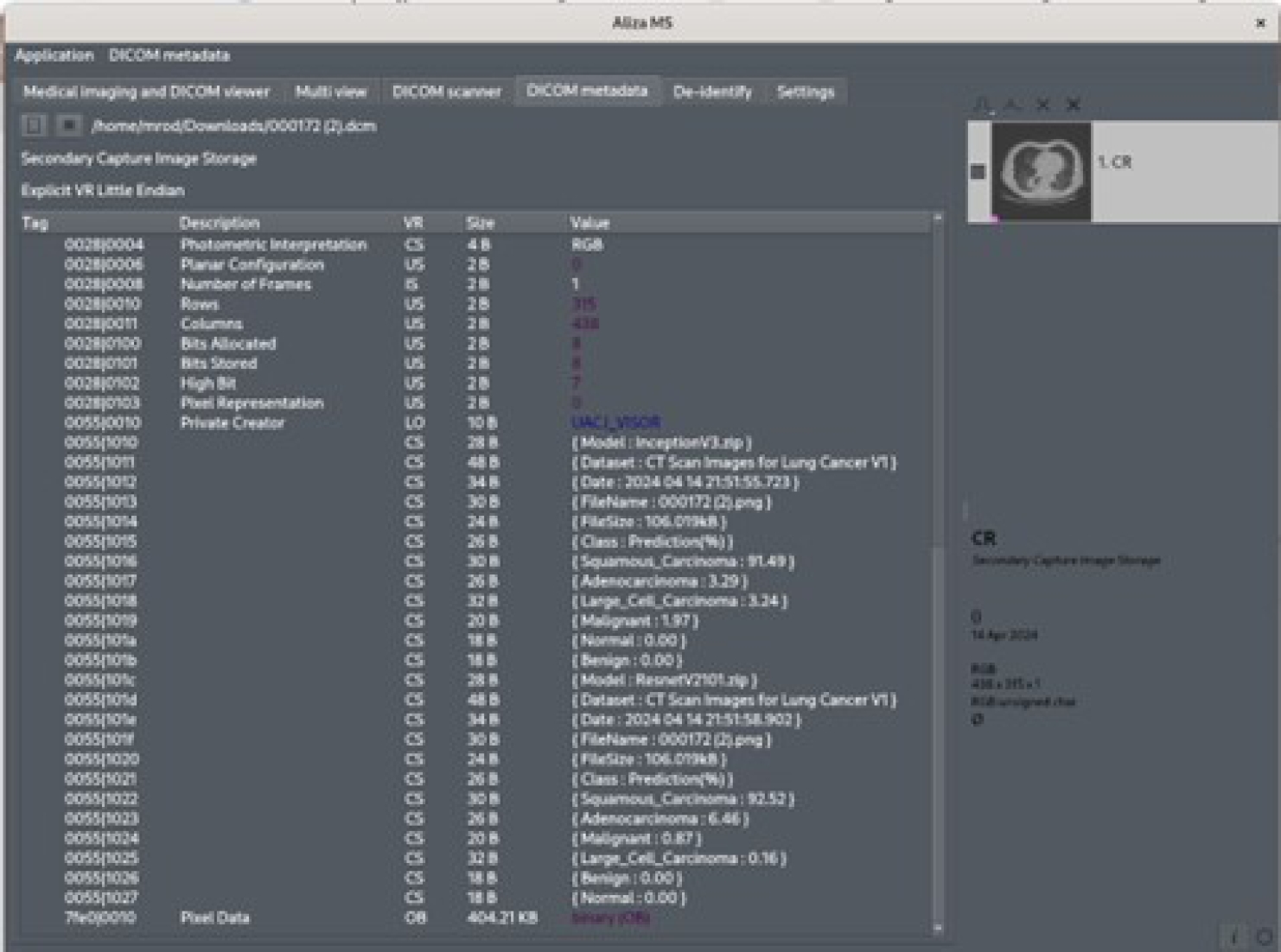
Because the predicted results are stored under the DICOM standard, these are also available to other DICOM viewers. Figure 18 shows these values in the Aliza MS application. The Figure 19 shows them in the MicroDicom viewer.
3.4 Implementation of Deep Learning Models
In this section, the implementation of CNNs using transfer learning is presented. The implemented models were InceptionV3, MobileNetV2, Res-NetV2101 and ResNetV250, which are available in the ML.NET library. The models were trained with the following parameter settings, Epoch-100, BatchSize-25, LearningRate-0.01, TestFraction-0.3, and TrainFraction-0.7.
This parameter configuration is done in ML.NET code. With these TestFraction and TrainFraction parameters, the subsets for testing and training contain 430 images and 1030 images, respectively. The Microsoft Visual Studio 2022 Community version was used to perform the transfer learning process, which integrates the Model Builder option to leverage pre-trained machine learning models included in ML.NET.
The tasks performed in ML.NET include binary classification, multiclass classification, image classification, text classification, regression, recommendation, and forecasting. The transfer learning process was performed for the four models and involved the six steps described below:
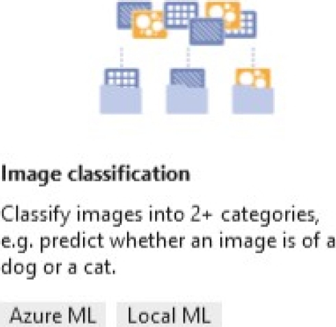
Selection of the scenario: The first step in initiating the transfer learning process was to select the task. Figure 20 shows the selection of the image classification task locally through Model Builder.
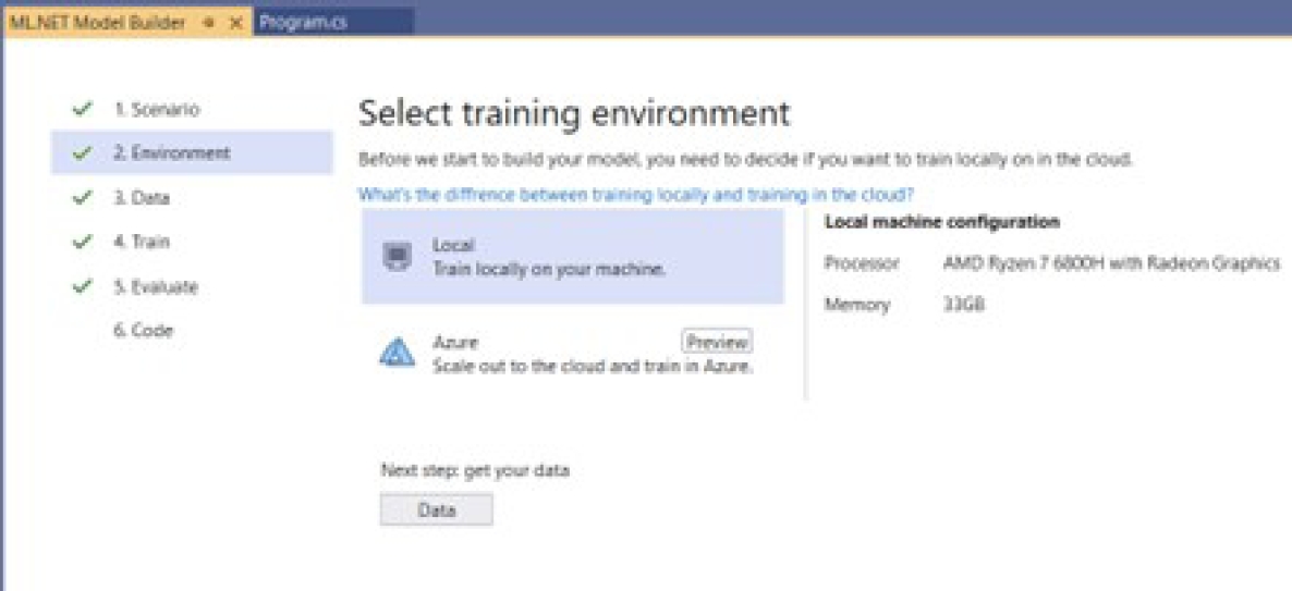
Selection of the training environment: In this step, the following options are available: local graphics processing unit (GPU), local central processing nit (CP), and the cloud with Microsoft Azure services, as shown in Figure 21. The local option was selected.
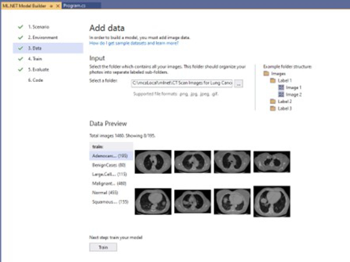
Add dataset: In this step, we select the path where the database containing the CT medical images with lung cancer is stored, as illustrated in Figure 22.
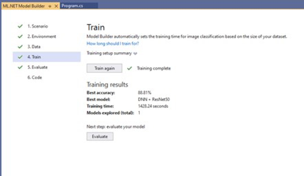
Train the model: In this step, the pre-trained model will now be trained with the selected database. The training process takes place once the model is chosen, as shown in Figure 23.
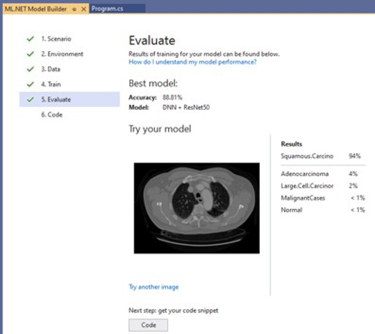
Evaluation model: Once the model is trained, its evaluation is carried out. Figure 24 presents an example of how the results of a model are shown; this model reached an accuracy of 88.81%. It also shows the percentage probability of having the diseases represented by each class: 94% Squamous.Carcinoma, 4% Adenocarcinoma, 2% Large.Cell.Carcinoma, less than 1% Malignant, and less than 1% Normal. The label is not displayed when the probability is too small, as with Benign.
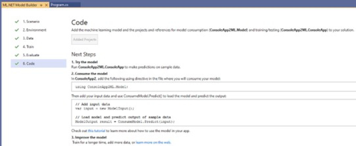
Code: Once the model is trained and its performance is known, it can be re-used. For this, Model Builder provides three options: (1) Console App, which allows it to be reused in a console application, (2) Web API, which allows it to be reused in a web application, and (3) the generation of a Notebook. This is shown in Figure 25. The developer determines the option to use. The chosen option was the Console App.
3.5 Interaction Between Learning Models and DICOM
The architecture implementation relies on open-source software such as Microsoft’s .NET libraries, C# libraries from fo-dicom on the server-side, and JavaScript libraries like jQuery.js and Dojo.js for client-side development, as shown in Figure 26. The server and client interaction is established through a web socket, allowing bidirectional communication.
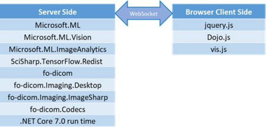
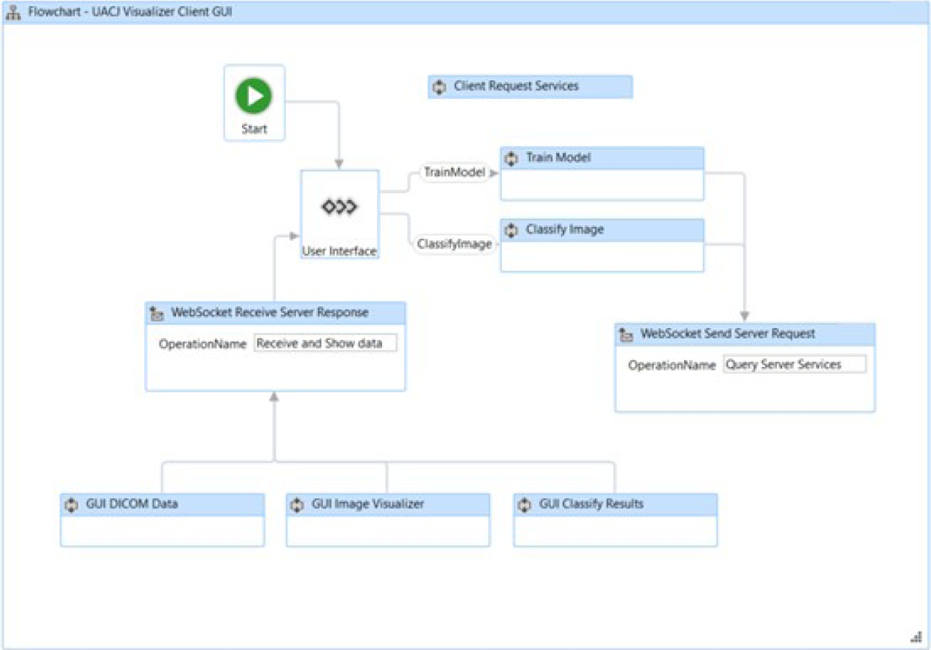
This means that the server can send notifications to the connected user without waiting for the client to send a communication request. In this structure, the server trains the selected TensorFlow model and makes predictions of image pathologies; the client displays the image and the model prediction results to the viewer. The interaction between the server and the client is shown in Figure 27.
The server-side application is composed of three classes: the Model class, BuildDicom class, and Server class, as shown in Figure 28. The Model class contains the methods and logic for training the desired model.
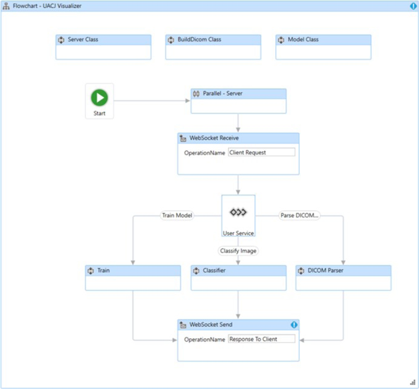
The BuildDicom class contains the methods for interpreting DICOM tags. This class implements editing both standard tags and private tags. It also incorporates the ability to process more than one image per file, known as multi-frame imaging.
The Server class describes the multiprocessing method that serves each user connected through a web socket. The user interface of the developed viewer shows the private elements (0055, xxxx) described in Table 3. Figure 29 shows the user interface of the viewer.
4 Results
This section presents the results obtained from the proposed architecture. Section 4.1 describes the results obtained by each of the models. Section 4.2 shows the structure of the DICOM viewer. Lastly, Section 4.3 describes the steps to classify a medical image or DICOM file.
4.1 Results Obtained
The performance achieved by each of the trained models is presented below. The reported metrics are AccuracyMacro, AccuracyMicro, Recall, Precision, LogLoss, and the Confusion Matrix and the Classification Report are also provided.
For all trained models, the LogLoss value is better the closer it is to zero. For Precision and Recall, a value closer to one is better. We ran each model ten times per dataset.
The results with higher microAccuracy values are presented below. It is worth mentioning that the tables and figures of the results presented in this section were generated by the viewer developed in this work. Tables 4 and 5 present InceptionV3 image distribution files. Tables 6 and 7 display the metrics for the training accuracy (Accuracy) and test accuracy (microAccuracy).
Table 4 InceptionV3 CT scan images of lung cancer image distribution
| Class | Train | Test | Total |
| Adenocarcinoma | 147 | 48 | 195 |
| Benign | 55 | 25 | 80 |
| Large_Cell_Carcinoma | 81 | 34 | 115 |
| Malignant | 316 | 144 | 460 |
| Normal | 316 | 139 | 455 |
| Squamous_Cell_Carcinoma | 115 | 40 | 155 |
| Total (Images) | 1030 | 430 | 1460 |
| Size (MB) | 134.36 | 59.07 | 193.43 |
Table 5 InceptionV3 IQ-OTHNCCD lung cancer image distribution
| Class | Train | Test | Total |
| Benign | 90 | 30 | 120 |
| Malignant | 393 | 168 | 561 |
| Normal | 293 | 123 | 416 |
| Total (Images) | 776 | 321 | 1097 |
| Size (MB) | 111.12 | 46.52 | 157.63 |
Table 6 InceptionV3 CT scan images of lung cancer metrics
| Metric | Value |
| Accuracy | 0.9942 |
| microAccuracy | 0.9163 |
| macroAccuracy | 0.8471 |
| LogLoss | 0.3053 |
| LogLossReduction | 0.8047 |
Table 7 InceptionV3 IQ-OTHNCCD lung cancer metrics
| Metric | Value |
| Accuracy | 0.9923 |
| microAccuracy | 0.9657 |
| macroAccuracy | 0.9373 |
| LogLoss | 0.1309 |
| LogLossReduction | 0.8589 |
Figure 30 shows the plots obtained for the accuracy and loss. Tables 8 and 10 display confusion matrices. Tables 9 and 11 show the classification reports. Tables 12 and 13 present MobileNetV2 image distribution files. Tables 14 and 15 display the metrics for the trainig accuracy (Accuracy) and test accuracy (microAccuracy).
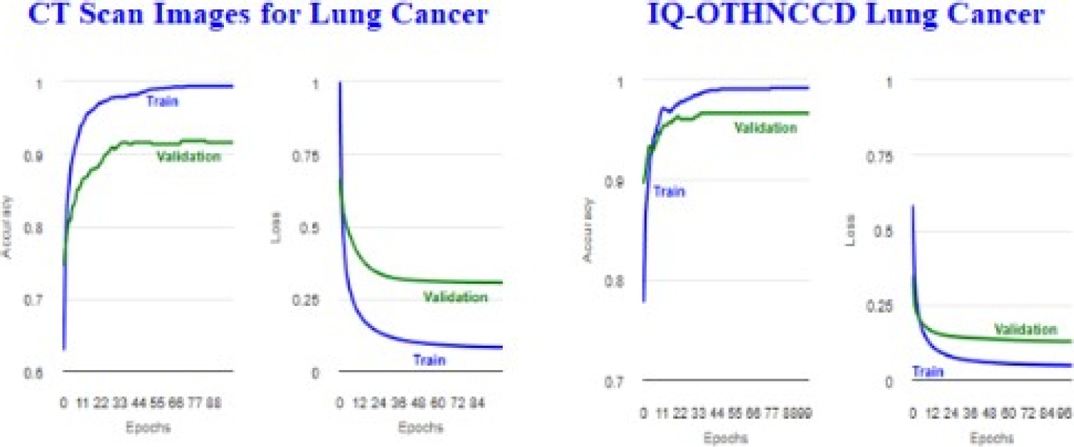
Table 8 InceptionV3 CT scan images of lung lancer confusion matrix
| Class-Truth | 0 | 1 | 2 | 3 | 4 | 5 | Recall | LogLoss |
| 0 | 37 | 0 | 3 | 2 | 1 | 5 | 0.7708 | 0.8114 |
| 1 | 0 | 19 | 0 | 2 | 4 | 0 | 0.76 | 0.6629 |
| 2 | 3 | 0 | 28 | 0 | 0 | 3 | 0.8235 | 0.905 |
| 3 | 0 | 0 | 0 | 144 | 0 | 0 | 1 | 0.0363 |
| 4 | 0 | 3 | 0 | 0 | 136 | 0 | 0.9784 | 0.0997 |
| 5 | 7 | 0 | 2 | 0 | 1 | 30 | 0.75 | 0.6467 |
| Precision | 0.7872 | 0.8636 | 0.8485 | 0.973 | 0.9577 | 0.7895 |
Table 9 InceptionV3 CT scan images of lung cancer classification report
| Class | Precision | Recall | F1-score | Support |
| Adenocarcinoma | 0.7872 | 0.7708 | 0.7789 | 48 |
| Benign | 0.8636 | 0.76 | 0.8085 | 25 |
| Large_Cell_Carcinoma | 0.8485 | 0.8235 | 0.8358 | 34 |
| Malignant | 0.973 | 1 | 0.9863 | 144 |
| Normal | 0.9577 | 0.9784 | 0.968 | 139 |
| Squamous_Cell_Carcinoma | 0.7895 | 0.75 | 0.7692 | 40 |
| Accuracy | 0.9163 | 430 | ||
| Macro avg | 0.8699 | 0.8471 | 0.8578 | 430 |
| Weighted avg | 0.914 | 0.9163 | 0.9148 | 430 |
Table 10 InceptionV3 IQ-OTHNCCD lung cancer confusion matrix
| Truth | Class | 0 | 1 | 2 | Recall | LogLoss |
| 0 | Benign | 26 | 0 | 4 | 0.8667 | 0.6534 |
| 1 | Malignant | 0 | 167 | 1 | 0.994 | 0.0163 |
| 2 | Normal | 6 | 0 | 117 | 0.9512 | 0.1599 |
| precision | 0.8125 | 1 | 0.959 |
Table 11 InceptionV3 IQ-OTHNCCD lung cancer classification report
| Column1 | Precision | Recall | F1-score | Support |
| Benign | 0.8125 | 0.8667 | 0.8387 | 30 |
| Malignant | 1 | 0.994 | 0.997 | 168 |
| Normal | 0.959 | 0.9512 | 0.9551 | 123 |
| Accuracy | 0.9657 | 321 | ||
| Macro avg | 0.9238 | 0.9373 | 0.9303 | 321 |
| Weighted avg | 0.9668 | 0.9657 | 0.9662 | 321 |
Table 12 MobileNetV2 CT scan images of lung cancer image distribution
| Class | Train | Test | Total |
| Adenocarcinoma | 143 | 52 | 195 |
| Benign | 52 | 28 | 80 |
| Large_Cell_Carcinoma | 86 | 29 | 115 |
| Malignant | 324 | 136 | 460 |
| Normal | 313 | 142 | 455 |
| Squamous_Cell_Carcinoma | 112 | 43 | 155 |
| Total (Images) | 1030 | 430 | 1460 |
| Size (MB) | 133.47 | 59.96 | 193.43 |
Table 13 MobileNetV2 IQ-OTHNCCD lung cancer image distribution
| Class | Train | Test | Total |
| Benign | 86 | 34 | 120 |
| Malignant | 404 | 157 | 561 |
| Normal | 286 | 130 | 416 |
| Total (Images) | 776 | 321 | 1097 |
| Size (MB) | 111.05 | 46.59 | 157.63 |
Table 14 MobileNetV2 CT scan images of lung cancer metrics
| Metric | Value |
| Accuracy | 0.997 |
| microAccuracy | 0.9116 |
| macroAccuracy | 0.8422 |
| LogLoss | 0.2656 |
| LogLossReduction | 0.8314 |
Table 15 MobileNetV2 IQ-OTHNCCD lung cancer metrics
| Metric | Value |
| Accuracy | 0.999 |
| microAccuracy | 0.9595 |
| macroAccuracy | 0.887 |
| LogLoss | 0.1247 |
| LogLossReduction | 0.8693 |
Figure 31 shows the plots obtained for the accuracy and loss. Tables 16 and 18 display confusion matrices. Tables 17 and 19 show the classification reports. Tables 20 and 21 present ResNetV2101 image distribution files.
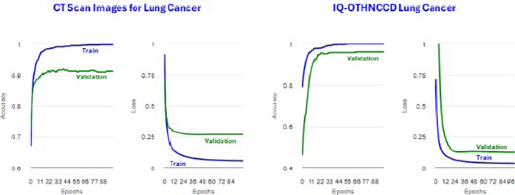
Table 16 MobileNetV2 CT scan images of lung cancer confusion matrix
| Class-Truth | 0 | 1 | 2 | 3 | 4 | 5 | Recall | LogLoss |
| 0 | 45 | 1 | 3 | 0 | 0 | 3 | 0.865 | 0.416 |
| 1 | 0 | 18 | 0 | 0 | 10 | 0 | 0.643 | 0.776 |
| 2 | 3 | 0 | 22 | 0 | 0 | 4 | 0.759 | 0.5 |
| 3 | 0 | 1 | 0 | 131 | 4 | 0 | 0.963 | 0.157 |
| 4 | 0 | 2 | 0 | 0 | 140 | 0 | 0.986 | 0.071 |
| 5 | 6 | 0 | 1 | 0 | 0 | 36 | 0.837 | 0.578 |
| precision | 0.833 | 0.818 | 0.846 | 1 | 0.909 | 0.837 |
Table 17 MobileNetV2 CT scan images of lung cancer classification report
| Class | Precision | Recall | F1-score | Support |
| Adenocarcinoma | 0.8333 | 0.8654 | 0.8491 | 52 |
| Benign | 0.8182 | 0.6429 | 0.72 | 28 |
| Large_Cell_Carcinoma | 0.8462 | 0.7586 | 0.8 | 29 |
| Malignant | 1 | 0.9632 | 0.9813 | 136 |
| Normal | 0.9091 | 0.9859 | 0.9459 | 142 |
| Squamous_Cell_Carcinoma | 0.8372 | 0.8372 | 0.8372 | 43 |
Table 18 MobileNetV2 IQ-OTHNCCD lung cancer confusion matrix
| Class | Column2 | 0 | 1 | 2 | Recall | LogLoss |
| 0 | Benign | 23 | 0 | 11 | 0.676 | 0.824 |
| 1 | Malignant | 0 | 157 | 0 | 1 | 0.002 |
| 2 | Normal | 2 | 0 | 128 | 0.985 | 0.089 |
| precision | 0.92 | 1 | 0.921 |
Table 19 MobileNetV2 IQ-OTHNCCD lung cancer classification report
| Class | Precision | Recall | F1-score | Support |
| Benign | 0.92 | 0.6765 | 0.7797 | 34 |
| Malignant | 1 | 1 | 1 | 157 |
| Normal | 0.9209 | 0.9846 | 0.9517 | 130 |
| Accuracy | 0.9595 | 321 | ||
| Macro avg | 0.947 | 0.887 | 0.9104 | 321 |
| Weighted avg | 0.9595 | 0.9595 | 0.9571 | 321 |
Table 20 ResNetV2101 CT scan images of lung cancer image distribution
| Class | Train | Test | Total |
| Adenocarcinoma | 138 | 57 | 195 |
| Benign | 57 | 23 | 80 |
| Large_Cell_Carcinoma | 84 | 31 | 115 |
| Malignant | 319 | 141 | 460 |
| Normal | 324 | 131 | 455 |
| Squamous_Cell_Carcinoma | 108 | 47 | 155 |
| Total (Images) | 1030 | 430 | 1460 |
| Size (MB) | 137.8 | 55.63 | 193.43 |
Table 21 ResNetV2101 IQ-OTHNCCD lung cancer image distribution
| Class | Train | Test | Total |
| Benign | 90 | 30 | 120 |
| Malignant | 396 | 165 | 561 |
| Normal | 290 | 126 | 416 |
| Total (Images) | 776 | 321 | 1097 |
| Size (MB) | 111.18 | 46.45 | 157.63 |
Tables 22 and 23 display the metrics for the training accuracy (Accuracy) and test accuracy (microAccuracy). Figure 32 shows the plots obtained for the accuracy and loss. Tables 24 and 26 display confusion matrices. Tables 25 and 27 show the classification reports.
Table 22 ResNetV2101 CT scan images of lung cancer metrics
| Metric | Value |
| Accuracy | 0.993 |
| microAccuracy | 0.907 |
| MacroAccuracy | 0.8242 |
| LogLoss | 0.2478 |
| LogLossReduction | 0.8435 |
Table 23 ResNetV2101 IQ-OTHNCCD lung cancer metrics
| Metric | Value |
| Accuracy | 0.981 |
| microAccuracy | 0.9377 |
| MacroAccuracy | 0.8631 |
| LogLoss | 0.1675 |
| LogLossReduction | 0.82 |
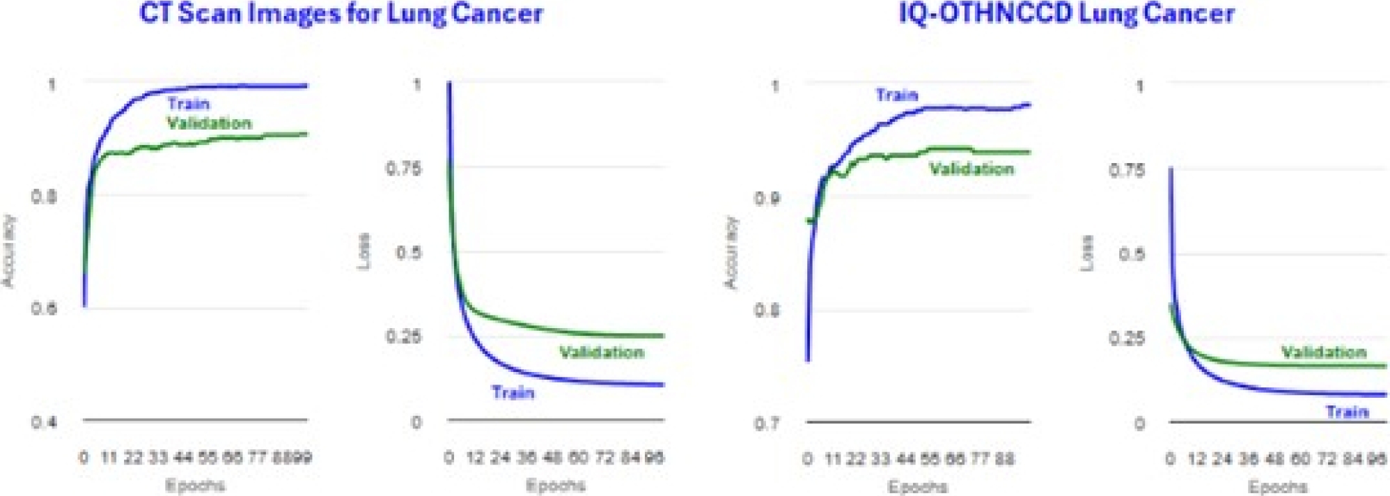
Table 24 ResNetV2101 CT scan images of lung cancer confusion matrix
| Class-Truth | 0 | 1 | 2 | 3 | 4 | 5 | Recall | LogLoss |
| 0 | 47 | 0 | 3 | 0 | 0 | 7 | 0.825 | 0.476 |
| 1 | 0 | 14 | 0 | 1 | 8 | 0 | 0.609 | 0.834 |
| 2 | 4 | 0 | 21 | 1 | 0 | 5 | 0.677 | 0.948 |
| 3 | 0 | 0 | 0 | 140 | 1 | 0 | 0.993 | 0.039 |
| 4 | 0 | 4 | 0 | 0 | 127 | 0 | 0.97 | 0.076 |
| 5 | 4 | 0 | 1 | 1 | 0 | 41 | 0.872 | 0.328 |
| precision | 0.854 | 0.778 | 0.84 | 0.979 | 0.934 | 0.774 |
Table 25 ResNetV2101 CT scan images of lung cancer classification report
| Class | Precision | Recall | F1-score | Support |
| Adenocarcinoma | 0.8545 | 0.8246 | 0.8393 | 57 |
| Benign | 0.7778 | 0.6087 | 0.6829 | 23 |
| Large_Cell_Carcinoma | 0.84 | 0.6774 | 0.75 | 31 |
| Malignant | 0.979 | 0.9929 | 0.9859 | 141 |
| Normal | 0.9338 | 0.9695 | 0.9513 | 131 |
| Squamous_Cell_Carcinoma | 0.7736 | 0.8723 | 0.82 | 47 |
| Accuracy | 0.907 | 430 | ||
| Macro avg | 0.8598 | 0.8242 | 0.8382 | 430 |
| Weighted avg | 0.9055 | 0.907 | 0.9046 | 430 |
Table 26 ResNetV2101 IQ-OTHNCCD lung cancer confusion matrix
| Truth | Class | 0 | 1 | 2 | Recall | LogLoss |
| 0 | Benign | 20 | 1 | 9 | 0.667 | 0.677 |
| 1 | Malignant | 1 | 164 | 0 | 0.994 | 0.038 |
| 2 | Normal | 8 | 1 | 117 | 0.929 | 0.215 |
| precision | 0.69 | 0.988 | 0.929 |
Table 27 ResNetV2101 IQ-OTHNCCD lung cancer classification report
| Class | Precision | Recall | F1-score | Support |
| Benign | 0.6897 | 0.6667 | 0.678 | 30 |
| Malignant | 0.988 | 0.9939 | 0.9909 | 165 |
| Normal | 0.9286 | 0.9286 | 0.9286 | 126 |
| Accuracy | 0.9377 | 321 | ||
| Macro avg | 0.8687 | 0.8631 | 0.8658 | 321 |
| Weighted avg | 0.9368 | 0.9377 | 0.9372 | 321 |
Tables 28 and 29 present ResNetV250 image distribution files. Tables 30 and 31 display the metrics for the training accuracy (Accuracy) and test accuracy (microAccuracy). Figure 33 shows the plots obtained for the accuracy and loss. Tables 32 and 34 display confusion matrices.
Table 28 ResNetV250 CT scan images of lung cancer image distribution
| Class | Train | Test | Total |
| Adenocarcinoma | 136 | 59 | 195 |
| Benign | 62 | 18 | 80 |
| Large_Cell_Carcinoma | 90 | 25 | 115 |
| Malignant | 331 | 129 | 460 |
| Normal | 316 | 139 | 455 |
| Squamous_Cell_Carcinoma | 95 | 60 | 155 |
| Total (Images) | 1030 | 430 | 1460 |
| Size (MB) | 136.03 | 57.4 | 193.43 |
Table 29 ResNetV250 IQ-OTHNCCD lung cancer image distribution
| Class | Train | Test | Total |
| Benign | 87 | 33 | 120 |
| Malignant | 392 | 169 | 561 |
| Normal | 297 | 119 | 416 |
| Total (Images) | 776 | 321 | 1097 |
| Size (MB) | 112.3 | 45.34 | 157.63 |
Table 30 ResNetV250 CT scan images of lung cancer metrics
| Metric | Value |
| Accuracy | 0.991 |
| microAccuracy | 0.9163 |
| macroAccuracy | 0.8633 |
| LogLoss | 0.262 |
| LogLossReduction | 0.8333 |
Table 31 ResNetV250 IQ-OTHNCCD lung cancer metrics
| Metric | Value |
| Accuracy | 0.991 |
| microAccuracy | 0.9626 |
| macroAccuracy | 0.8934 |
| LogLoss | 0.1156 |
| LogLossReduction | 0.877 |
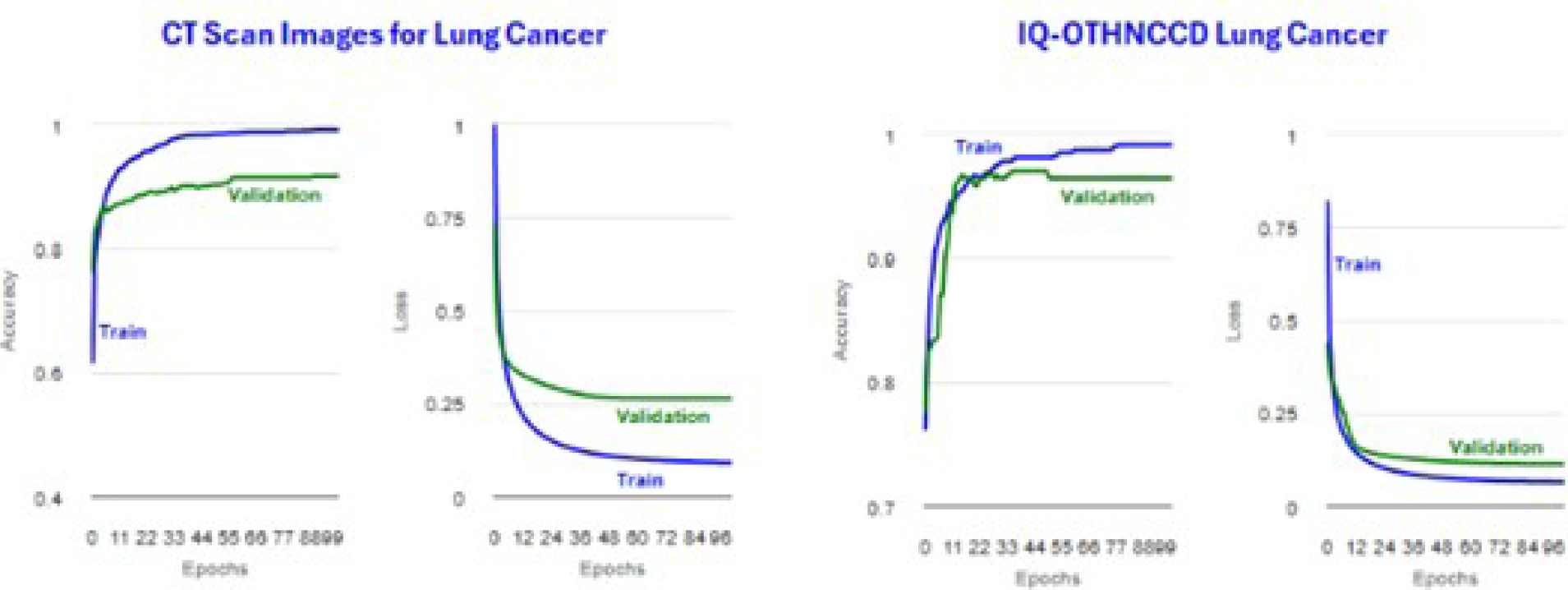
Table 32 ResNetV250 CT scan images of lung cancer confusion matrix
| Class-Truth | 0 | 1 | 2 | 3 | 4 | 5 | Recall | LogLoss |
| 0 | 46 | 0 | 1 | 1 | 1 | 10 | 0.78 | 0.654 |
| 1 | 0 | 14 | 0 | 1 | 3 | 0 | 0.778 | 0.839 |
| 2 | 2 | 0 | 20 | 0 | 0 | 3 | 0.8 | 0.545 |
| 3 | 0 | 0 | 0 | 127 | 2 | 0 | 0.984 | 0.048 |
| 4 | 0 | 3 | 0 | 1 | 135 | 0 | 0.971 | 0.072 |
| 5 | 6 | 0 | 2 | 0 | 0 | 52 | 0.867 | 0.487 |
| precision | 0.852 | 0.824 | 0.87 | 0.977 | 0.957 | 0.8 |
Table 33 ResNetV250 CT scan images of lung cancer classification report
| Class | Precision | Recall | F1-score | Support |
| Adenocarcinoma | 0.8519 | 0.7797 | 0.8142 | 59 |
| Benign | 0.8235 | 0.7778 | 0.8 | 18 |
| Large_Cell_Carcinoma | 0.8696 | 0.8 | 0.8333 | 25 |
| Malignant | 0.9769 | 0.9845 | 0.9807 | 129 |
| Normal | 0.9574 | 0.9712 | 0.9643 | 139 |
| Squamous_Cell_Carcinoma | 0.8 | 0.8667 | 0.832 | 60 |
| Accuracy | 0.9163 | 430 | ||
| Macro avg | 0.8799 | 0.8633 | 0.8707 | 430 |
| Weighted avg | 0.9161 | 0.9163 | 0.9157 | 430 |
Table 34 ResNetV250 IQ-OTHNCCD lung cancer confusion matrix
| Truth | Class | 0 | 1 | 2 | Recall | LogLoss |
| 0 | Benign | 23 | 2 | 8 | 0.697 | 0.63 |
| 1 | Malignant | 0 | 169 | 0 | 1 | 0.025 |
| 2 | Normal | 2 | 0 | 117 | 0.983 | 0.102 |
| Precision | 0.92 | 0.988 | 0.936 |
Tables 33 and 35 show the classification reports. Tables 36 and 37 summarize the model metrics. We observe that for CT Scan Images for the Lung Cancer dataset, the positive prediction percentage is above 90.0%.
Table 35 ResNetV250 IQ-OTHNCCD lung cancer classification report
| Class | Precision | Recall | F1-score | Support |
| Benign | 0.92 | 0.697 | 0.7931 | 33 |
| Malignant | 0.9883 | 1 | 0.9941 | 169 |
| Normal | 0.936 | 0.9832 | 0.959 | 119 |
| Accuracy | 0.9626 | 321 | ||
| Macro avg | 0.9481 | 0.8934 | 0.9154 | 321 |
| Weighted avg | 0.9619 | 0.9626 | 0.9604 | 321 |
Table 36 Metrics of deep learning methods on CT scan images for lung cancer dataset
| Metric | InceptionV3 | MobileNetV2 | ResNetV2101 | ResNetV250 |
| Accuracy | 0.994 | 0.997 | 0.993 | 0.991 |
| microAccuracy | 0.9163 | 0.9116 | 0.907 | 0.9163 |
| MacroAccuracy | 0.8471 | 0.8422 | 0.8242 | 0.8633 |
| LogLoss | 0.3053 | 0.2656 | 0.2478 | 0.262 |
| LogLossReduction | 0.8047 | 0.8314 | 0.8435 | 0.8333 |
Table 37 Metrics of deep learning methods on IQ-OTHNCCD lung cancer dataset
| Metric | InceptionV3 | MobileNetV2 | ResNetV2101 | ResNetV250 |
| Accuracy | 0.992 | 0.999 | 0.981 | 0.991 |
| microAccuracy | 0.9657 | 0.9595 | 0.9377 | 0.9626 |
| MacroAccuracy | 0.9373 | 0.887 | 0.8631 | 0.8934 |
| LogLoss | 0.1309 | 0.1247 | 0.1675 | 0.1156 |
| LogLossReduction | 0.8589 | 0.8693 | 0.82 | 0.877 |
The ResNetV2101 model obtained the lowest value of 90.7%, while the ResNetV250 model achieved the highest value of 91.63%, InceptionV3 obtained 91.63%; and MobileNetV2 obtained 91.16%. Even though InceptionV3 and ResNetV250 have the same value, the difference in the accuracy value is bigger for InceptionV3. Thus, we can conclude that these models have a good prediction performance.
For the IQ-OTHNCCD Lung Cancer dataset, the positive prediction percentage is above 93.70%. The InceptionV3 model obtained the highest value of 96.57%, and ResNetV2101 had the lowest value of 93.77%. MobileNet ob-tained 95.95%, while ResNetV250 obtained 96.26%.
4.2 Medical Image DICOM Viewer
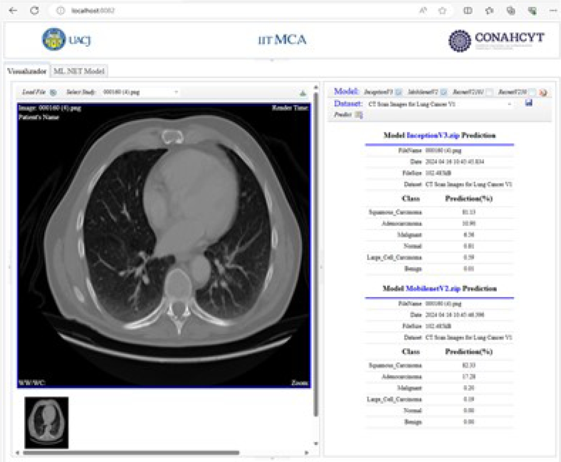
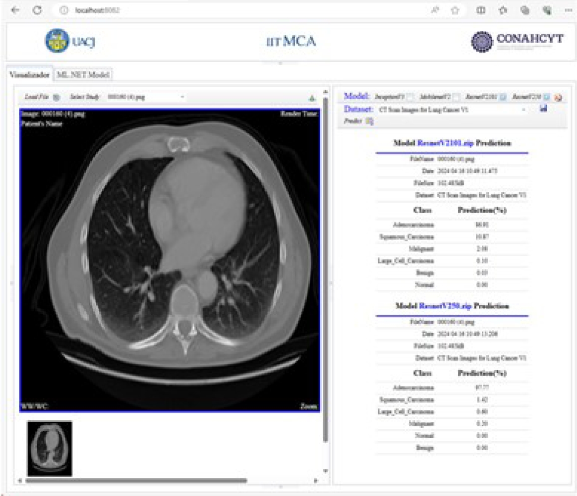
After the training and evaluation phase, the predictions of the models are displayed using the DICOM standard. Figure 34 shows the prediction results of the pre-trained InceptionV3 and MobileNetV2 models. Figure 35 shows the prediction results of the pre-trained ResNetV2101 and ResNetV250 models.
4.3 DICOM Viewer User Interface
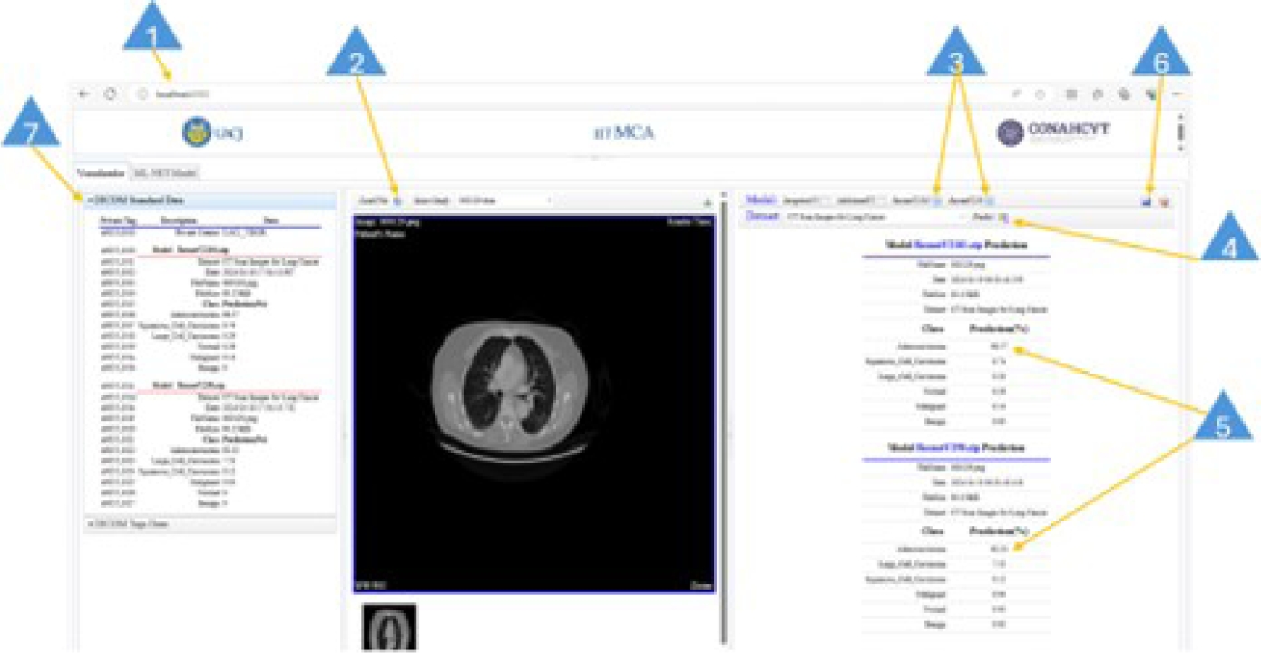
The DICOM viewer user interface is easy to use. It does not require users to have deep knowledge of deep learning, data science, or computer science. Figure 36 shows the DICOM viewer user interface. The basic steps to perform a prediction task are given below:
Type in the web address of the viewer.
Click the Load File button to load an image file (JPG/PNG format) or a DICOM file (.dcm extension).
Select the model or models for the prediction task. This is achieved by clicking on the check box on the model task bar.
Click the Predict button to run the prediction process. This will take a few seconds to finish.
This step involves reading the reported values. The closer they are to 100%, the higher the probability that the pathology is present for this image.
Click on the disk icon to save the obtained results. This creates or updates a DICOM-format file, which including the private element x0055, 0010.
The DICOM file tags are available on the DICOM Standard Data panel.
5 Conclusion
In this research, we present the architecture of a decision support method to assist radiologists in diagnosing pathologies in medical images, focusing on detecting lung cancer with six different pathology classes. Our proposed architecture integrates a) deep learning models, b) custom private DICOM tags, and c) a viewer that displays classification results stored in DICOM private tags. The DL models InceptionV3, MobileNetV2, ResNet2101, and ResNetV250 were trained using TensorFlow ML algorithms supported in Microsoft’s ML.NET library on the CT Scan Images for Lung Cancer and IQ-OTHNCCD Lung Cancer datasets.
The CT Scan Images for Lung Cancer dataset consists of 1,460 images, with 70% (1030 images) used for training and 30% (430 images) for testing. The IQ-OTHNCCD Lung Cancer dataset is composed of 1,097 images, providing 776 images for training and 321 images for testing using a test fraction of 0.3.
The results show that all the models have an excellent prediction performance above 90%. We added the DICOM private element x0055 to store the prediction results of each trained DL model. The prediction results are displayed for the radiologist and patient through a graphical interface. The graphical interface consists of two main code blocks, one for the client-side application implemented in JavaScript and the other for the server-side application implemented in C#. The proposed architecture shows that it can support radiologists as a second opinion.
In future work, we consider extending the architecture to datasets related to other pathologies. Additionally, algorithms for image analysis can be integrated to perform analysis and add annotations to the image, plus evaluate image quality, resolution, blur, and visibility, among other characteristics. An important future step is to get support and feedback from domain experts (radiologist personnel), as this is necessary to validate the generated prediction results, which should match radiologist’s expected results.

