


 nueva página del texto (beta)
 Inglés (pdf)
 Artículo en XML
 Referencias del artículo
 Enviar artículo por email
 Citado por SciELO
  Similares en
SciELO
Similares en
SciELO 
 Permalink
1 Introduction
It is widely known that there are a variety of methods to measure the randomness of the samples produced by pseudo-random number generators. As an example, some of these methods are: Frequency test, Gap test, Poker test, Run test, Serial test, Coupon collector's test, Permutation test, Maximum of t test, Collision test, Chi-Square test, Kolmogorov–Smirnov test, Autocorrelation test, and the Spectral test, among other methods.
The operating mechanism of the existing methods, as well as their benefits, are mentioned in various sources [2-4, 9, 12].
However, all these methods have the drawback of measuring only some particular aspects of pseudo-random series, that is, in their statistical analysis they do not treat the series as a whole; then, it may be the case that, with some of such methods, many generators succeed in passing randomness tests, but not with all methods, which leads to the assumption that these methods are not always suitable for measuring randomness.
On the other hand, it is clear that the construction of pseudo-random generators implies, among other tasks, dealing with factors such as 1. The periodicity or presentation of cycles, which is unavoidable in most pseudo-random generators, if not in all.
To highlight this situation, Table 1 shows some of the C++ 11 random class generators [9]. Therefore, if you want to develop an application for cryptographic purposes, these generators are not an option 2.
Table 1 Characteristics of some pseudo-random generators included in C++11 [3,9]
| Name | Predictability | Performance | State | Period |
| Mersenne Twister | Trivial | OK | 2KiB | 2^1937 |
| LOG(minstd) | Trvial | OK | 4-8 byte | <=2^32 |
| LFG | Trivial | Slow | 8-16 byte | <=2^32 |
| Knuth | Trivial | Super slow | 1KB | <=2^32 |
| Ranlux | Unknown | Super slow | *120byte | 10^17 |
The predetermined production of pseudo-random series, which occurs in all generators of a mathematical nature, in which a seed, also determined, produces a pseudo-random series known in advance. 3. The Pseudo-random generators’ speed of performance, in addition to being dependent on considerations of uniformity, security and independence, are also dependent on response time.
Table 1 [9] shows that speed can be a weakness, as is the case for two of the engines presented in that table.
For the reasons mentioned, this paper proposes a method with the aim of contributing to the search for more robust randomness indicators, which allow not only the evaluation of the generators, but also lead to the construction of better pseudo-random generators.
This method was given the name Comprehensive Method for Measuring Randomness in Pseudorandom Generators, CMMRPG, and its design is based on the fact that sequences must be available where the generation of these numbers is almost uniform and independent.
Before explaining the CMMRPG, it is necessary to mention that over the years a variety of test protocols have also appeared, each one combining several methods to measure randomness, among these protocols: KNUTH Protocol that combines the Birthday Spacings tests, Collision test, Coupon collector´s test, Frequency test, Gap test, Maximum-of-t test, Permutation test, Poker test, Run test, Serial test and Serial correlation test; DIEHARD Protocol that combines the Binary Rank tests (31x31,32x32 and 6x8 matrices), Birthday Spacings tests, Bitstreams test, Counts-the-1´s test (for streams and for bytes), Craps test, DNA tests, Minimum distance tests, Overlapping permutations test, Overlapping sums test, Overlapping pairs sparse occupancy test, Overlapping-quadruples-sparse-occupancy test, Parking Lot test, Random spheres test, Run test and Squeeze test; DIEHARDER Protocol that combines all test in Diehard plus the GDC test of Marsaglia-Tsang, Generalized minimum distance test, Lagged sums test, the Permutation test, Monobit test, Run test, the Generalized serial test, the Bit distribution and Kolmogorov-Smirnov test; NIST-15 Protocol that combines Approximate entropy test, the Binary Matrix Rank test, Cumulative sums test, Discrete Fourier Transform test, Frequency test, Frequency within a block test, Linear Complexity test, Maurer's universal statistical test, Non overlapping template matching test, Overlapping template matching test, Random excursions variant test and Serial test; HELSINKI Protocol that combines the Autocorrelation, Cluster test, n-block test and Random walk test; ENT Protocol that combines the Arithmetic mean, Chi square test, Entropy test, Monte-Carlo Pi estimation test and Serial correlation test; Crypt-X Protocol which combines the Binary derivative test, Change point test, Frequency test, Linear complexity test, Run test and Sequence complexity test; SPRING Protocol that combines the Collision test, Coupon Collector´s test, Fourier test, Frequency test, Transform test, Gap test, the Ising Model, Maximum-of-t test, Permutation test, Poker test, Random walk test, Run test and Serial test.
The Diehard test protocol and the NIST 800-22 currently stand out, among the existing protocols above. They are described next:
1.1 Diehard Test Protocol
The Diehard protocol [10, 17] consists of a set of tests that, for the most part, returns a p-value, which should be uniform on the interval (0,1) if the input sequence contains truly independent random bits. Those p-values are obtained by p=F(X), where F is the distribution of the random variable X, often a normal function. But F is just an asymptotic approximation, for which the fit will be worse on the tails of the function.
Therefore, we should not be surprised that p-values close to 0 or 1 occasionally appear. When a sequence of bits fails conspicuously, p-values of 0 or 1 will be obtained at many places in the sequence. Since many tests are done, it is likely to find some p<0.025 or some p>0.975, which does not mean that the random number generator fails the test at the 0.05 level.
However, the Diehard protocol does not generate a unified criterion that involves all the tests in a single indicator that measures the random quality of a sample.
1.2 NIST 800-22 Test Protocol
The NIST 800-22 test protocol [2, 10, 13], is a suite for randomness analysis, generally used for formal certifications. These tests, like those of the Diehard protocol, analyze various aspects of a sequence of pseudo-random numbers, and have the particularity of being focused on the evaluation of pseudo-random generators intended for cryptographic tasks. Like the DIEHARD protocol, it does not generate a unified indicator for the analyzed data series.
This paper emcompass the Introduction, Section 2, that defines the elements that give rise to the generation of pseudo-random numbers by the generator used in this investigation. Section 3, presents the proposal to use the byte to measure the randomness of pseudo-random generators. Section 4 mentions the pseudo-random generator used in this investigation. Section 5 shows, step by step, how the randomness index proposed in this research is constructed. Section 6 explains the tests performed. Section 7 summarizes an analysis of the results. Section 8 shows the most relevant conclusions of this research.
2 Precursors
In this research, the term precursors refer to all the physical events that can be used in the creation of random data, since they are events that precede and give rise to these data. And these data, although they can be called random, at the moment in which the mechanism of occurrence of their precursors is known, they pass into the category of pseudo-random.
On the other hand, today's pseudo-random number generators use number seeds as precursors. Being, by definition, these generators, mathematical-statistical models, whether they are of the type of congruential methods or of another type, which means that they are within the algorithms that Von Newman defined as algorithms that are in "sin", because in no way they generate really random data [6].
Similarly, it is known that we are surrounded by situations where the outcome is quite uncertain, and surely the only thing we can do, a priori, is to assign probabilities to each outcome in the state space of these situations. Therefore, any event whose occurrence is determined by models of complexity superior to the comprehension of human knowledge can be considered random in nature.
So, in this context, and as a way of justifying the use of the definition of precursors, we can consider as valid precursors unexpected natural events such as earthquakes, solar flares, hailstorms and others that cannot be predicted with precision, and that hit the different regions of the planet.
Similarly, in the usual computer equipment, we have variables that are provided by the hardware/software of the system, such as the ticks of the clock, the identification number assigned to a process, the system time at the time of executing a routine and the GUIDs (globally unique identifiers) that can be generated alternately with the readings of other temporary variables.
In any case, and regardless of the context, for a precursor to be eligible as such, any of their multiple’s states must have a probability of occurrence close to 1/N, where N is the number of values that cover the state space of the precursor. It is desirable to have as many valid precursors as possible, in order to build a number generator that meets the standards of sufficient randomness. In this research, events generated by the computer are used as precursors.
3 Measure Randomness Using Data Bytes
It is known that, in order to measure the randomness of a data sequence produced by a pseudo-random number generator, common methods proceed to statistical analysis of the bits that make up that data sequence [7, 14-15]. In this research, we worked with the byte instead of the bit, the main motivation for using this unit being the fact that it can represent intelligible entities for humans, such as a letter, a number, a special character, etc.
Another advantage of making randomness measurements with bytes is that the analysis is done on 256 different values, and not on two different values as when working with bits. For example, suppose that a random generator, whose output is given in bits, generates 24 consecutive 1s digits. This fact allows us to assume a bias, or even a serious failure in the pseudo-random production of the generator. In contrast, if the output is in bytes, three consecutive bytes with the value 255 do not raise the same concern as 24 consecutive equal bits. On the other hand, a graphical, or visual, interpretation of the curves formed by the 256 numbers is more reliable, precisely, because they are formed by a greater variety of data.
4 Random Number Generator Used
The tests of the proposed CMMRPG were carried out on pseudo-random sequences produced by a generator, also novel, which is the product of another investigation carried out by the authors of this paper. This generator is not described in this paper because its operation is being evaluated in another scientific journal, however, its high performance can be highlighted, constituted by a great randomness in the numbers produced. For the purposes of this paper, this generator will be called the Cylinder Mechanism.
This generator, if given the precursors of the type ticks of the computer system clock, the identification number assigned to the process by the operating system, the time of executing a routine, the GUIDs, events of pressing keys, from mouse movements and any other precursors that are not under the user's control; it can produce sequences with very high levels of randomness, which is an ability that makes it superior to the more popular generators [16], and well suited for use in cryptography.
5 Construction of the Randomness Index, RI
This index, obtained through CMMRPG, is built following both the Independence criterion and the data uniformity criterion [1,10, 11, 12], and it works with the bytes of the sequences as proposed in section 3.
The RI construction process begins with the calculation of the following statistics: the Intermedian Comparator (defined as part of this investigation), the arithmetic mean, the median, the standard deviation, the autocorrelation, the interquartile coefficients (defined as part of this investigation), the variation coefficient, the concentration coefficient (defined as part of this investigation), the appearance coefficient (defined as part of this investigation), the correlation index (defined as part of this investigation), the interquartile frequency distribution (defined as part of this investigation), Gap Test Randomness Index and the Index provided by the Test of repetitions (REPI) (defined as part of this investigation).
Next, the proposed statistics are defined, differentiating between those that determine the uniformity and those that determine the independence of the data.
5.1 Components to Calculate the Uniformity of Frequency Distribution of the Sequences
Data uniformity is addressed with the following components:
Intermedian Comparator (IC): This measure is obtained by comparing the sum of the frequencies on both sides of the median. So, if m is the median, LSS is the sum of the frequencies on the left side of m and RSS is the sum of the frequencies on the right side of m. If f(i) is the frequency at each element of the range of n elements, then LSS and RSS are determined as:
The IC is defined in the range
Interquartile Comparators (P12, P23 and P34): These measures consider the frequencies on both sides of the quartiles.
Let now be the following values:
P1: sum of frequencies of the data with a value lower than quartile 1 (Q1).
P2: sum of frequencies of the data between quartile 1 and quartile 2 (Q2).
P3: sum of frequencies of the data between quartile 2 and quartile 3 (Q3).
P4: sum of frequencies of the data with a value greater than quartile 3 (Q3).
Namely:
In the same way that the IC is calculated, P12, P23 and P34 are calculated, but considering the frequencies of both sides of each quartile:
Concentration Coefficient (CC): Measures how clustered the data is around the mean. For which the Coefficient of Variation (CV) is used:
And the CC is defined as CC = 1 – CV.
Appearance Coefficient (AC): This coefficient is established to search for abnormalities in the distribution of the data, which the other coefficients mentioned above cannot detect. For example, that a number never appears, rarely or many times. That is, that its appearance value is below the mean minus 3 standard deviations or exceeds the mean value plus 3 standard deviations. That range is known to pool 99.7% of the data in a normal distribution.
AC is calculated by assigning each frequency value f(i) a rating C(i), with 0≤i ≤255.
Let be the mean frequency X and the standard deviation σ, the C(i) are obtained, for the different values of f(i), as follows:
If f(i) ≥ 2X ⇒ C(i) = 0
If f(i) > X+3σ ∧ f(i) < 2X ⇒ C(i) = (2X–f(i))/(X-3σ)
If f(i) ≥ X-3σ ∧ f(i) ≤ X+3σ ⇒ C(i) = 1
If f(i) ≤ X-3σ ⇒ C(i) = f(i)/ (X - 3σ)
Once all the C(i) have been calculated, the AC is obtained as:
Interquartile frequency distribution (IFD): This measure was defined to establish if the frequency, of the values in the range 0-255, is distributed homogeneously on both sides of each quartile. Each quartile has a size of n/4, where n is the total size of the sample. To calculate this measure, first must be obtained the sum of the frequencies, for each value 0-255, within the limits of each quartile.
Now, for each frequency there are four values or quantities that denotes its appearances within each quartile. With these four values must be calculated the mean frequency F and the standard deviation. There is, then, a set of pairs (Fi, σi), for 0≤ i≤255.
For each pair (Fi, σi), the coefficient of variation CVi is calculated, thus, 256 coefficients of variation are obtained, as shown in Eq. 8, with n=255.
Of these 256 coefficients of variation, the one with the highest value is selected:
Finally, we have:
5.2 Components to Calculate the Independence of the Sequence Data
Data independence is addressed with the following components.
Autocorrelation (A) [5, 8]: It is well known that autocorrelation is a very useful tool to measure the independence of data. Let's remember its equation:
where:
N: It is the size of the data sequence.
h: It is the interval of the regressors.
X: Arithmetic mean of the data sequence.
Xi: the i-th data of the sequence.
The A has a maximum value of 1.0 and a minimum value of 0.0. Lower values correspond to more randomness of the data sequence and values close to 1.0 represent less randomness. This made it necessary to define the Correlation Index CI = 1.0 – A. Which makes the correlation criterion close to 1 mean more randomness, to be in line with the uniformity indices of section 5.1.
Gap Test Randomness Index (GAPI): to calculate this component of value 0 and 1, the Gap Test was used. Digit sequences were used, and once the gap intervals were established, the Kolmogorov-Smirnov test was used [10-11, 18].
The procedure for calculating the GAPI is as follows:
Let D* = Dcalculated and D = Dreliability
As it is known, if Dcalculated < Dreliability, the digits appear randomly ordered, and if Dcalculated >
Dreliability, the digits are not randomly ordered.
For a given sequence of digits, we record the number of times the gaps of lengths 0, 1, 2, … appear. After noting how often each gap occurs, the observed relative cumulative frequency (Sx) is compared to the theoretical cumulative frequency F(x).
Assuming that the digits are randomly ordered, the relative cumulative frequency distribution is given by:
where m is the frequency of the GAP and T, the Total GAPs. The theoretical cumulative frequency distribution is given by:
Theoretically, the frequency distribution for randomly ordered digits is given by:
Let us see an example. If a level of significance Sig = 0.05 is adopted, and the following sequence of digits is obtained:
2, 9, 3, 1, 6, 3, 0, 4, 6, 3, 2, 8, 7, 0, 8, 1, 3, 1, 8, 3, 6, 0, 7, 9, 6, 1, 3, 4, 8, 6, 3, 4, 9, 1, 4, 2, 8, 1, 0, 5, 5, 9, 2, 3, 1, 4, 0, 5, 8, 8, 9, 8, 3, 9, 9, 3, 3, 5, 9, 1, 1, 5, 3, 6, 8, 4, 7, 7, 9, 6, 0, 4, 0, 6, 0, 5, 7, 3, 1, 5, 9, 5, 4, 0, 1, 4, 6, 0, 0, 5, 4, 6, 2, 4, 8, 4, 2, 0, 5, 4, 4, 1, 0, 2, 0, 5, 4, 1, 3, 7, 5, 3, 3, 1, 6, 7, 1, 0, 2, 9, 6, 7, 0, 1, 7.
The GAPs number recorded will be the number of digits analyzed minus the number of different random digits generated (in this case, the digits 0 to 9, that is, 10 digits). Total Gaps is T=N–10, where N=125 is the number of digits analyzed. So, T = 125 –10 = 115.
Then, the longest gap length is checked, and the required intervals are determined. For example, if you have a gap length equal to 49, and you want 10 intervals, then the first interval will be 0–4, the second 5–9, the third 10–14, etc. Conversely, if only 5 intervals are required, then the first interval would be 0–9, the second 10–19, the third 20–29, the fourth 30–39, and the fifth 40–49.
For the example sequence, the largest gap length is 50, and that sequence was divided into 17 intervals. Subsequently, each of the generated random numbers is analyzed to determine its gap length and obtain the frequency in the generated intervals. Thus, selecting the digit 7, its first gap length is 9; and it will fall in the interval 9–11, then that interval will have its first occurrence.
If the same digit or another digit falls in that same interval, then the second occurrence for this interval would be added; and so on for all intervals. The sum of the occurrences, of all the intervals, is equal to the Total GAPs (T=115).
Gap test steps:
The probability function for the theoretical frequency distribution is specified, given by Eq. 14, using the width of the selected intervals.
The observed gaps in a cumulative distribution with the same intervals are tabulated.
Calculate D*, the maximum deviation, in absolute value, between F(x) and Sn(x) as in Eq. 15.
The critical value Dα, from the Kolmogorov– Smirnov table, is determined for the specific value of α and the sample size N.
If D* calculated is greater than Dα, it is concluded that there is no independence of the data, that is, GAPI=0:
FA (Cumulative Frequency = Sn(x)) is calculated with Eq. 16:
For the example sequence:
FA of the interval (0–2) = (27 /115) = 0.234.
FA of the interval (3–5) = (57 /115) = 0.495.
FA of the interval (6–8) = (80 /115) = 0.695.
FA of the interval (9–11) = (91 /115) = 0.792.
FA of the interval (…) = (…) = …
(…) = (...) = ...
Fx are calculated as follows:
Fx(0–2) = 1 – (0.9)2+1 = 0.271
Fx(3–5) = 1 – (0.9)5+1 = 0.469
Fx(6–8) = 1 – (0.9)8+1 = 0.613
Fx(9–11) = 1 – (0.9)11+1 = 0.718
Fx(…) = ...
… = …
The absolute maximum difference between FA and Fx, was, for this test, 0.082* as shown in Table 2. The absolute maximum difference is compared with the reliability difference (Dα), which is given by Eq. 18:
Table 2 Calculation of frequencies and differences for the gap text
| Gap size | OC | FA Sn(x) | Frecuencies Fx(x) | |Fx(x) - Sn(X)| |
| 0 - 2 | 27 | 0.234 | 0.271 | 0.037 |
| 3 - 5 | 30 | 0.495 | 0.469 | 0.026 |
| 6 - 8 | 23 | 0.695 | 0.613 | 0.082 * |
| 9 - 11 | 11 | 0.792 | 0.718 | 0.074 |
| 12 - 14 | .... | ........ | .......... | ... ... ... |
In Table 2, a sample of the results of the described example is presented. Where FA and OC are the cumulative frequency and the occurrence in each interval, respectively. The rows following the range 9–11 are omitted as these are not relevant to explaining the results of this example.
Applying a reliability level α=0.95, there is a significance level Sig=0.05, and as the sample size N>35, then, the value in the Kolmogorov-Smirnov table [18] is 1.36, therefore, Dα(0.95)=0.127. Since D*=0.082 < Dα=0.127, we conclude that the sequence of digits for this example is random. That is, GAPI=1.
Index by the Test of repetitions (REPI):
This test, which is done on digits, is designed to determine how many times the same repeated digit appears in partial sequences of 4, 5, 6 repetitions, in a large sequence of digits.
For example, it can be expected that in a sequence of 100 digits there will be up to 20 partial sequences of 5 repetitions of the same digit. Of course, if the sample is evenly distributed, that's not going to happen. When a random wheel of digits 0-9 spins, each digit has a 1/10 chance of appearing, but that doesn't mean that if it is spun 10 times, every single digit will appear.
It is possible, that in a set of 40 spin actions, the digit 1 only appears once and the digit 5 appears 4 times, and so on with the other digits. If the number of experiments is large enough, the occurrences of the digits tend to follow a uniform distribution.
There is a sample with N digits generated by a pseudo-random engine and these are stored in an array from position 0 to position N-1. Position 1 is set as the start of the experiment. Here, it is worth asking how likely it is that the digit 2 is equal to the digit 1?
Each digit has a 1/10 chance of appearing. If the test is done in position 0, there will be a probability of 1/10 that the digit in that position is equal to the one in position 1. Therefore, there is a probability 9/10×9/10 = 81/100 that the digit in position 1 is a non-repeating digit (i.e. is an isolated digit).
It was observed, when consecutive tests were carried out on 100,000,000 digits, that, on average, 80,999,639 digits were no repeated contiguously, a value very close to that calculated with Eq. 19.
For this case, 100,000,000× (81/100)= 80,999,999. For partial sequences of repetitions of 2, 3, 4, 5, 6 or more digits, divide the result of Eq. 19, among 10 successively, as shown in Table 3.
Table 3 Ideal appereances Over 100 million digits
| Appeareance | Expected | |
| Isolated digits: | Expected[0] | 80,999,999 |
| Pairs: | Expected[1] | 8,0999,99 |
| Triples: | Expected[2] | 809,999 |
| Quartrains: | Expected[3] | 80,999 |
| Quintets: | Expected[4] | 8,099 |
| Sextets: | Expected[5] | 809 |
| Septets: | Expected[6] | 80 |
| Octets: | Expected[7] | 8 |
| 9 repetitions: | Expected[8] | 0 |
A decrease given by a factor of 10 is observed as more digits are grouped. This was experimentally confirmed with the results shown in Table 4. This is mathematically logical given that each digit added to a previous grouping has a 1/10 chance of appearing.
Table 4 Occurrences observed for pseudo-random Cylinder Mechanism and C++ 11 intdistro () generators
| Appeareances | Cylinders mechanism | intdistro() C++ |
| Isolated digits: | 80,993,170 | 81,006,197 |
| Pairs: | 8,102,948 | 8,097,687 |
| Triples: | 810,370 | 809,514 |
| Quartrains: | 80,946 | 80,989 |
| Quintets: | 8,021 | 8,124 |
| Sextets: | 786 | 787 |
| Septets: | 85 | 75 |
| Octets: | 8 | 7 |
| 9 repetitions: | 0 | 0 |
Table 3 shows the expected or theoretical occurrences over 100 million digits. Table 4 shows the occurrences observed over 100 million digits produced by the pseudo-random generators: Cylinder Mechanism and intdistro () of C++11.
An evident similarity of the results produced by the two pseudo-random generators is observed, and also, the similarity between the expected and observed repetitions produced by the two generators.
The differences between the expected and observed repetitions must be subject to a tolerance. That is, a number that measures how much the observed data can be allowed to deviate from the calculated quantities. That tolerance must first be defined for digits without contiguous repetitions.
Let:
Topdata: the maximum number of data to be analyzed, for this investigation was 1,000,000,000 digits.
Nr_data: the number of data of the sample to be analized, that has to be a multiple of 10. It is recommended to go from 106 to 109.
Maxdispersion: the tolerance that is allowed on the Topdata amount of data, equal to 0.0050 for one billion digits. That is, between the expected amount and the observed amount there can only be a difference of up to 50,000 occurrences in 1,000 million digits. The number 50,000 is called Tolerance.
Let
Let PT be the Previous Tolerance and ND be the Next_dispersion containing the value Maxdispersion/2, the Tolerance(Expected[i]) for i>0, is:
Now, let
In order to calculate the subsequent Tolerance(Expected[i]), where 1 ≤ i < Mag-2, we have the following algorithm:
Begin
Mag
Tolerance(Expected[0]]
PT
ND
For i =1 To i < Mag-2 Step 1
ND
Tolerance(Expected[i]
PT
End for
End
To qualify the repetition test, proceed as follows:
4 test protocols are executed: 100 tests on 1,000,000 digits, 100 on 10,000,000, 100 on 100,000,000 and 100 on 1,000,000,000 digits, respectively. The total number of failed tests is added and the REPI index is obtained by eq. 22.
5.3 Proposed Randomness Index
Finally, the IC, P12, P23, P34, DC, AC, IFD, CI, GAPI and REPI components are combined to establish the RI:
This index has the advantage that any bias, of some importance, in any of the components will be reflected in the result, which is an indication that the randomness of the series being analyzed is compromised in one or several of its components precursors, or that the generator is not an efficient mechanism.
6 Convergence Tests of the RI
A wide variety of tests were carried out, of which four large blocks are described.
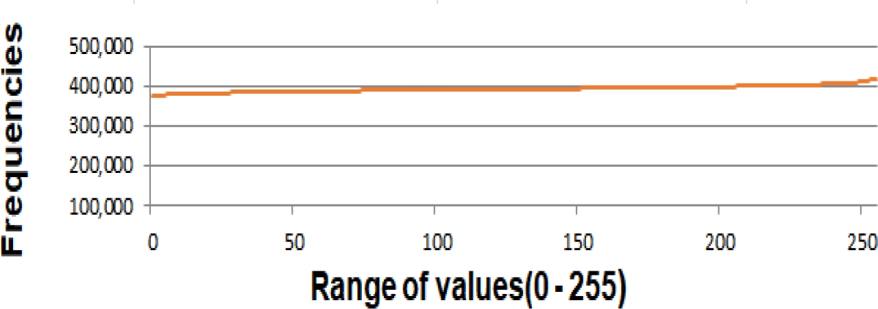
6.1 Block of 100 Runs: Each Run with a Pseudo-Random Sequence of one Million Data
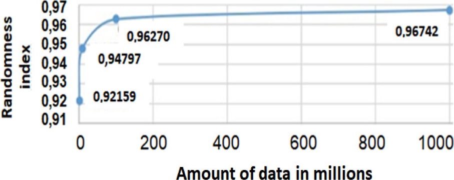
The average statistics obtained for this block are: Mean: 392.156,8627451, Median: 398.758, Deviation: 7.973,9140445, A: 0,030035, LSS: 50.193.128,000, RSS: 49.806.872,000, IC: 0,9923046, P1: 25.196.104,500, P2: 24.797.644,500, P3: 24.748.348,500, P4: 24.859.144,500, P12: 0,984, P23: 0,998, P34: 0,996, CC: 0,979, AC: 1, IFD = 0,992618 CI: 0,9782020, GAPI = 1, REPI =1 and finally, RI=0.92159.
Fig. 1 shows the average frequency distribution of the 256 values present in the pseudo-random sequences used in this run block.
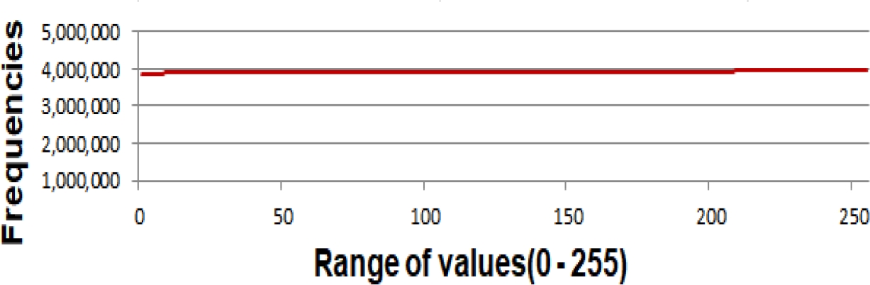
6.2 Block of 1000 Runs: Each Run with a Pseudo-Random Sequence of one Million Data
The average statistics obtained for this block are:
Mean: 392.156,8627451, Median: 392.036,600, Deviation: 2.027,724, A: 0,029985, IC: 0,999954968613, CV: 0,00517069619, P12: 0,9834359, P23: 0,9992262, P34: 0,9997221, CC: 0,9948311627, AC: 1, IFD = 0,992618 CI: 0,9772225, GAPI =1, REPI=1 and finally, RI=0,94797.
Fig. 2 shows the average frequency distribution of the 256 values present in the pseudorandom sequences used in this run block.
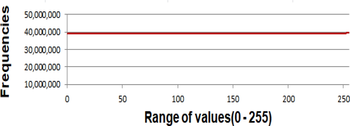
6.3 Block of 10000 Runs: Each Run with a Pseudo-Random Sequence of One Million Data
The average RI for this block of runs turned out to be 0.96270. Fig. 3 shows the average frequency distribution of the 256 values present in the pseudo-random sequences used in this run block.
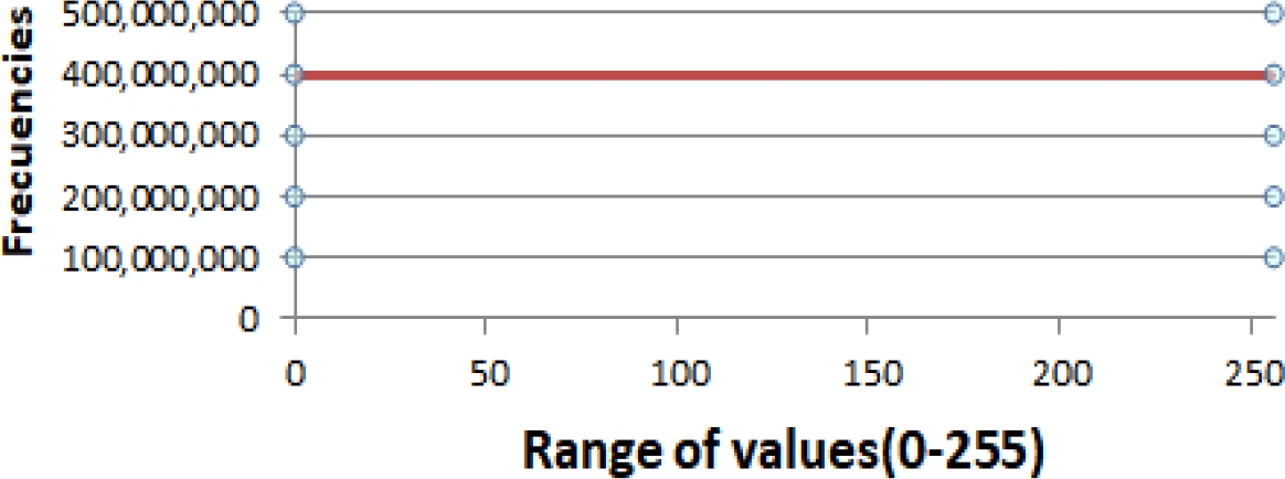
6.4 Block of 100000 Runs: Each Run with a Pseudo-Random Sequence of One Million Data
The average RI for this block of runs turned out to be 0,96742. Fig. 4 shows the average frequency distribution of the 256 values present in the pseudo-random sequences used in this run block.
7 Analysis of the Results
In all the tests carried out, an almost uniform distribution of the data was observed, as can be seen in figures 1, 2, 3 and 4.
Fig. 5 shows the convergence of the standard deviation to zero as the increases the volume of data.
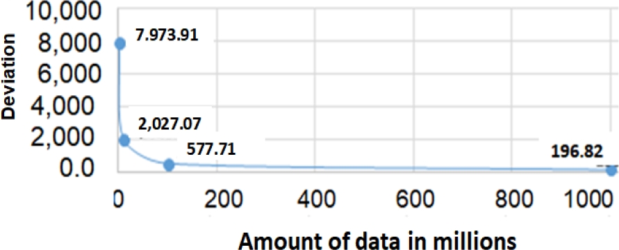
Fig. 6 shows a convergence of the RI to 0.97, which means that the Cylinder Mechanism is an excellent pseudo-random numbers generator, with random quality.
8 Conclusions
The RI is a good measure of the random ability of any generator. In this investigation it was possible to validate its robustness because it worked with the Cylinder Mechanism, which is a high-performance generator and the intdistro() pseudo-random generator of the C++ 11 language.
The tests showed that the Cylinder Mechanism, too, is a robust generator since uniformity and independence of the data could be observed in the range 0-255. The use of precursors is an efficient strategy to achieve the performance capacity of the used pseudo-random number generator. The proposed RI is very robust against popular randomness measurement methods.
The proposed RI defines the level of randomness based on the mixture of many statistics, which makes it very reliable. The statistics defined as part of this research are adequate to build the proposed RI.
Popular pseudo-random generators could, in some cases, deliver higher rates, but they being seed-dependent, making them unsuitable for cryptographic uses.
In this investigation, the RI increased with the amount of data, which verifies the good performance of the Cylinder Mechanism.
The good performance of the Cylinder Mechanism, plus the varied use of precursors, during a test protocol constitute the best option to trigger the generation of pseudo-random numbers with high levels of randomness.
Finally, it can be concluded that the CMMRPG proposed in this paper constitutes a valid alternative to obtain robust randomness indicators and that, at the same time, allows the construction of robust pseudo-random generators.

