


 nueva página del texto (beta)
 Inglés (pdf)
 Artículo en XML
 Referencias del artículo
 Enviar artículo por email
 Citado por SciELO
  Similares en
SciELO
Similares en
SciELO 
 Permalink
1 Introduction
Nowadays, Embedded electronic systems have become ubiquitous in various sectors of activity, from transportation to healthcare, from consumer electronics to industrial automation.
One of the primary objectives of designing embedded electronic systems is to ensure their reliability and cost-effectiveness while performing complex tasks that meet the constraints of time, energy consumption, and manufacturing cost. Focusing on the scope of this paper, it is possible to mention as an example that flight plan planning algorithms used to find the shortest route or propose real-time avoidance trajectories incorporate sorting algorithms.
Indeed, sorting algorithms [29, 43, 1, 2] (sorts for short) play a vital role in the design and performance of embedded systems. In these systems, sorts are designed to meet the constraints of time and energy consumption. The choice of a sort depends on the nature of the data, the constraints, and the desired performance.
For example, bubble-sort or insertion-sort algorithms are easy to implement but are not suitable for large datasets or real-time applications. Conversely, quick-sort [37, 19], heap-sort [39], tim-sort [6, 22] and merge-sort [31, 19] algorithms are more complex and require more processing power but can handle large datasets and real-time applications. As technology continues to evolve, the demand for efficient and reliable embedded systems will only increase, and sorts will continue to play a vital role in meeting these demands.
Among these systems, FPGAs (Field-Programmable Gate Array) have emerged as an interesting alternative to accelerate software applications. FPGAs are integrated circuits that can be programmed to perform specific functions. They offer high performance and energy efficiency, making them suitable for real-time computing applications. Considering sorting operations, one approach is to use the FPGA’s built-in hardware resources to implement the sorts directly.
These algorithms can be optimized for the FPGA architecture, resulting in faster and more efficient sorting. Another approach is to use the FPGA to offload sorting operations from the CPU. In this approach, the CPU sends the data to be sorted to the FPGA, which sorts and returns the sorted data to the CPU.
This approach can significantly reduce the processing time required for sorting, as the FPGA can handle large data sets in parallel. One challenge in using FPGAs is the programming complexity since FPGA programming requires specialized knowledge in HDLs (Hardware Description Languages) such as Verilog and VHDL (very-high-speed integrated circuit hardware description language).
However, available tools and libraries can ease the programming process, making it more accessible to software developers. Moreover, CPUs can certainly be used in embedded systems. In many cases, embedded systems require a combination of processing power and low power consumption, which can be challenging to achieve with CPUs alone. To meet these requirements, CPUs are often used in conjunction with other components, such as FPGA’s microcontrollers, memories, communication interfaces, sensors, and other peripherals.
These components are integrated into a complete embedded system, which is designed to meet the specific needs of the application. The choice between CPUs and FPGAs really depends on the specific needs of the application. CPUs are great for applications that require flexibility and versatility, as they can be programmed to handle a wide range of tasks. On the other hand, FPGAs are designed for specific tasks, and are optimized for performance in those tasks.
This makes them ideal for applications that require high performance. While they may be more expensive to produce and harder to program than CPUs, their performance benefits can make them the best choice for some applications.
The objective of this paper is to compare optimized hardware and software implementations of heap-sort, shell-sort, quick-sort, tim-sort and merge-sort on FPGA and Intel i7 architectures using a limited number of elements ranging from 8 to 4096. Indeed, contrary to most of related works in the literature, there are 4096 elements at most because they are provided to a real-time decision support system as solutions to be sorted.
This is highlighted by the work of K. Nikolajevic [35], whose thesis aims to tackle the challenging problem of reducing operational accidents in avionics systems. As part of the collision avoidance alarm system, sorting these solutions efficiently is crucial for real-time decision making in avionics systems to select the best actions to avoid accidents.
To be more precise, each solution (i.e. a short-term path to follow in an avionics application) is identified by a unique 32-bit integer, so-called index, and evaluated on the basis of various performance criteria (such as distance...). Consequently, index-sorts are used in the real-life application. However, sorted elements constitute permutations of integers in this paper to simplify the problem. In general terms, the main contributions of this paper are as follows:
– Analysis and comparisons of the performance of five sorts: quick-sort, heap-sort, shell-sort, merge-sort, and tim-sort. Their performances are evaluated in terms of average and standard deviation of computational times on Intel i7 and FPGA architectures. These measurements are refined by statistical tests.
– Temporal stability analysis of the sorts: In addition to ranking the performance of the sorts on each platform, a statistical analysis is carried out on the basis of “boxplot-like” statistical measurements to assess the temporal stability of these algorithms.
The paper is structured as follows: Section 2 presents a state of the art on various sorts and several applications using different platforms (CPU, FPGA). Section 3 shows our experimental results. Section 4 gathers our conclusions and some of our future works.
2 Related Works
Over the past few decades, there has been a significant amount of research conducted on sorts. While many of these studies have focused on accelerating sorts in heterogeneous computing systems, there has also been a focus on reducing computational time, power consumption, and hardware resources. This literature review section provides an overview of numerous studies on both FPGA-based and CPU-based sorts that aim to improve acceleration performance.
2.1 Hardware Acceleration Methods for Embedded Systems (FPGA)
FPGAs are greatly flexible and customizable to meet the specific requirements of different applications. This flexibility allows FPGAs to be optimized either to perform high-performance parallel processing and data streaming in applications that require high throughput, or for fast response times in applications that require low latency, or finally for energy efficiency in applications that require low-power consumption.
The traditional development of FPGA-based applications has been mainly based on highly specialized register transfer level (RTL) designs [44, 18, 42, 5, 13, 34, 20]. High-Level Synthesis (HLS) allows increasing design productivity and detaching the algorithm from architecture [16]. In our case, the vivado HLS tool is used to generate hardware accelerators from C language.
Ben Jmaa et al. [9] proposed an efficient hardware implementation for different sorts using high-level descriptions in a zynq-7000 platform. The authors compared the performance of the algorithms in terms of computational time, standard deviation and resource utilization. The results showed that the selection-sort was 1.01-1.23 times faster than other algorithms for less than 64 elements; otherwise, tim-sort was the best algorithm. Kobayashi et al. [26, 27] detailed a new approach to reducing FPGA programming costs while maintaining high levels of performance.
Their sorting library can use OpenCL for FPGA. This approach consumed at least twice the hardware resources of the merge-sort method restructured for the OpenCL programming model for FPGA. However, it operated at a frequency 1.08 times higher and had a sorting throughput three orders of magnitude greater than the baseline.
Chen et al. [14] proposed a sample-sort algorithm on a server with a PCIe-connected FPGA to sort large data sets. The prototype system was implemented using Verilog HDL on Amazon Web Services (AWS) FPGA instances equipped with Xilinx Virtex UltraScale+ FPGAs.
The authors demonstrated that this system can sort 230 key-value records 37.4 times faster than GNU parallel sort running on a CPU with 8 threads. However, their method assumed collaboration between the CPU and FPGA, and the sorting performance was ultimately limited by the PCIe bandwidth, which was 7.2 GB/s as reported in [14]. Moreover, their method was not suitable for implementing FPGA-centric applications that require sorting due to its structure.
Shinyamada et al. [38] evaluated the impact of various sorts on high-level synthesized image processing hardware. The results showed that bubble-sort and odd-even-merge-sort were the fastest algorithms, as they were able to achieve pipeline processing. Conversely, selection-sort was not able to achieve ideal pipeline processing, and its performance was not as good as the former two algorithms. Concludingly, optimizing sorts can have a significant impact on overall image processing performance.
Moghaddamfar et al. [32] conducted a comparative analysis of OpenCL and RTL-based implementations of a heap-sort that merges sorted runs. The results showed that while both implementations required comparable development effort, their RTL implementations of critical primitives achieved four times better performance and used only half as much FPGA resources compared to the OpenCL implementation.
This highlighted the importance of carefully selecting the programming language and implementation approach when developing algorithms for FPGA-based systems. The study suggested that RTL-based implementations can provide significant performance benefits and resource efficiency compared to higher-level language implementations like OpenCL.
Chen et al. [15] proposed a novel hybrid pipelined sorting architecture based on a bitonic-sorter and several cascaded sorting units. This sorting architecture achieved a balanced trade-off between resource utilization and throughput, as well as between throughput and power consumption.
Specifically, the architecture was both resource and energy efficient in terms of the throughput-to-resource ratio and the throughput-to-power ratio. This study highlighted the importance of designing sorting architectures that maximize data parallelism to achieve increased throughput and reduced latency.
Montesdeoca et al. [33] monitored by a network of 40 CO2 sensors and performed real-time sorting of all the data via bubble-sort and insertion-sort on FPGA. The results showed that insertion-sort was faster than bubble-sort, but it consumed more hardware resources in the FPGA, illustrating the importance of the trade-off between speed and resource utilization when selecting a sort for real-time applications.
In [3], the authors evaluated multithreaded sorts on a 32-core reconfigurable architecture with embedded real-time Linux support. The architecture consisted of NIOS II/f soft cores and was implemented on an FPGA. The authors proposed a new approach for performance evaluation of a soft multithreaded multicore architecture conducted in real-time.
This approach was based on the recursive generation and execution of sorts such as merge-sort and quick-sort. The architecture was capable of achieving high parallelism and throughput while maintaining low latency. The architecture outperformed the others in terms of speed and scalability. In [1], the authors focused on hardware implementing bubble-sort, selection-sort, insertion-sort, merge-sort, bitonic-sort and odd-even-merge-sort using FPGA in synchronous and pipelined architectures. The authors compared these implementations in terms of computational time and area.
They showed that non-pipelined bitonic-sort and non-pipelined odd-even-merge-sort had the best performance in terms of computational time, while the non-pipelined selection-sort and non-pipelined insertion-sort had the lowest area of synchronous architecture.
For pipelined architectures, bitonic-sort and odd-even-merge-sort had much lower computational time when implemented in hardware. Additionally, odd-even-merge-sort was found to be the smallest in terms of area. While bitonic-merge-sort was slightly larger in area and slower in execution than odd-even-merge-sort.
Lobo et al. [31] compared five merge-sorts (serial-merge-sort, parallel-merge-sort, bitonic-merge-sort, odd-even-merge-sort and the modified-merge-sort) in terms of resource utilization, delay and area on FPGA. The results showed that the serial and parallel merge use the highest amount of resource utilization compared to bitonic-merge, odd-even-merge and modified-merge.
Also, the parallel-merge algorithm was much faster than a serial-merge algorithm. In addition, the odd-even and modified-merge had a very close value of the area used while bitonic-merge had as slightly higher value.
Abdelrasoul et al. [2] proposed an index and sort algorithm (IaSA) based on an FPGA (vertex-5 series) in a pipelined sequential structure using Verilog HDL. The results showed that, for various data set sizes, IaSA performed best in terms of computational time.
In [24], the authors presented a column-sort, mapped on an HBM (High Bandwidth Memory)-enabled FPGA. The approach utilized computational pipelines, hardware-efficient interconnection networks and several optimizations to achieve high-throughput sorting. The results showed that their optimized design yields 14.8×, 4.73× and 2.18× speedup compared with state-of-the-art implementations on CPU.
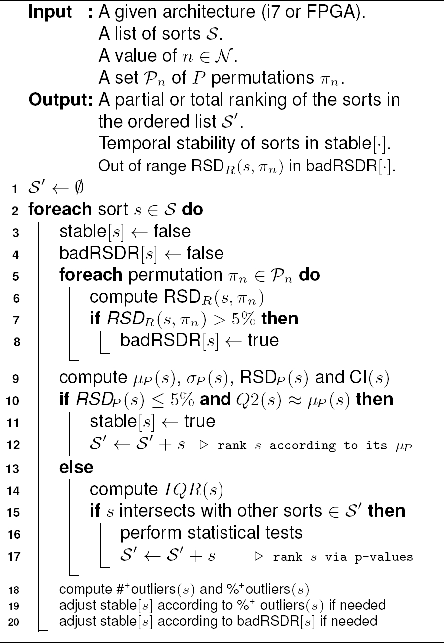
– Lines 5 to 8: First step of the algorithm, check for external variations from the computational environment.
– Line 8: badRSDR
– Lines 10 to 12:
– Line 10:
– Line 12:
CI
– Lines 13 to 17: In this step, statistical tests are required due to a high value of
– Line 15: Current confidence interval CI
– Line 16: Statistical tests are used to rank the sorts if possible, temporal stability tests of
– Line 17: At this point it is not always possible to strictly rank
– Lines 18 to 20: Check if sort
– Line 19: Set stable
– Line 20: Set stable
2.2 Software Acceleration Methods for Embedded Systems (ARM)
ARM processors offer advantages in terms of flexibility and ease of reconfigurable integration technology for a wide range of applications, from embedded systems to high-performance computing.
Compared to classical processors, soft-core processors like ARM allow for greater customization and adaptability because they can be easily programmed and reconfigured to meet the specific needs of a given application.
Additionally, soft-core processors can be integrated into a variety of reconfigurable technologies, such as FPGAs, allowing for even greater flexibility and performance optimization.
In [11, 10], the authors proposed a software implementation for insertion-sort, quick-sort, heap-sort, shell-sort, merge-sort, and tim-sort on an ARM Cortex A9. They compared the performance of these algorithms in terms of average and standard deviation of computational times, energy consumption, and temporal stability.
The results demonstrated that shell-sort was the best algorithm, being 42.1% faster and even reaching up to 72% faster when the number of elements to be sorted is greater than 64.
However, when the number of elements is smaller than 64, tim-sort was the best algorithm. Additionally, shell-sort was the best algorithm in terms of standard deviation of computational times and energy consumption.
In [7], the authors proposed a hardware heap-sort implementation using FPGA of a wavelet based image coder. Their architecture provided up to 20.9% power reduction on the memories compared to the baseline implementation. Moreover, their architecture provided 13x speedup compared to ARM Cortex A9.
In [8], the authors introduced an adaptive heap-sort that was designed for an image coding implementation on FPGA with high throughput and scalable sorting. The authors compared its performance to an embedded ARM Cortex A9 running at 666 MHz.
Their architecture, running at 100 MHz, provided around 13 times the speedup while consuming 242 mW of average core dynamic power. In [12], the authors adapted a hybrid sort based on quick-sort and bitonic-sort. They employed bitonic-sort to handle small partitions/arrays with a vectorized partitioning implementation to divide these partitions.
Their approach required only an array of size O(log n) for recursive calls in the partitioning phase. They evaluated the performance on an ARM v8.2 (A64FX) and assessed their implementation by sorting/partitioning integers, double floating-point numbers, and key/value pairs of integers. The results showed an average speedup factor of four compared to the GNU C++ sort algorithm.
In [25], the performance and energy efficiency of hardware and software implementations of the heap-sort are compared. The results showed that the hardware implementation (Digilent Basys 3 Artix-7 FPGA) was more energy efficient, but slower than software implementation (ARM Cortex A72) due to a low clock frequency.
2.3 Software Acceleration Methods for Non Embedded CPU
In “standard” workstations, Central Processing Units (CPUs) can drastically increase the number of instructions processed per second, allowing the computer to perform more complex tasks or run more programs simultaneously. Indeed, recent CPUs have a potential for higher performance thanks to higher clock speeds, more cores, and improved SIMD instructions. However, these processors consume much more power than their embedded counterparts.
In [30], the authors presented optimized serial and parallel counting-sorts. They compared this sort to others such as bucket-sort and merge-sort, implementing both counting-sort and merge-sort on CPU and GPU. The results showed that the optimized counting-sort took only 6 ms to sort 100 million integers, being 23 times faster than the previous version.
In [21], the authors provided an analysis of current host-GPU data transfer mechanisms and explored methods for mitigating performance bottlenecks. They developed a heterogeneous CPU/GPU sort and demonstrated that while out-of-place GPU sorting achieved the best performance, an in-place sort further reduced some host-side bottlenecks.
In [4], the authors compared the grouping-comparison-sort (GCS) to selection-sort, quick-sort, insertion-sort, merge-sort and bubble-sort, using random input sequences. On an Intel Core 2 Duo E8400 @ 3.00 GHz (2 CPUs), the result revealed that for small input sizes, the performance of all six algorithms was almost comparable.
However, for larger input, quick-sort proved to be the fastest, while selection-sort was the slowest. GCS ranked as the third fastest for small input size (10000 elements) and the fifth fastest for large input size (30000 elements). In [28], the authors introduced a distribution sorting method that utilized a trained model of the empirical Cumulative Distribution Function of the data.
Additionally, they applied a deterministic sort that performed well on almost sorted arrays, such as insertion-sort. The performance was measured on an Intel Xeon Gold 6150 @ 2.70 GHz using up to one billion double-precision keys following a normal distribution.
Their approach achieved an average performance improvement of 3.38 times compared to the C++ STL-sort, which is an optimized hybrid of quick-sort, a 1.49 times improvement over sequential radix-sort, and a 5.54 times improvement over a C++ implementation of tim-sort, which is the default sorting function for Java and Python.
2.4 Synthesis of Related Work
Table 1 summarizes a literature review focusing on the use of several sorts on different platforms (FPGA, Intel CPU, ARM). This summary shows that the authors generally use sorts on FPGA to improve performance in terms of computational time and resource usage. Moreover, a majority of authors do not use HLS except for [26, 27, 38, 9, 11, 10]. In addition, the number of elements to sort is usually much larger than thousands of items. Contrary to these studies, our work is based on different implementations of sorts using HLS and compare the sorts on FPGA and Intel i7 in terms of computational time, resources utilization and temporal stability.
Table 1 Review of sorting algorithms on different platforms
| Approach | Platforms | Algorithms | HLS | Optimization | Application domain | ||||
| Ref | FPGA | Intel CPU | ARM | Sort-name | Complexity | Perf. criteria | |||
| [26, 27] | Yes | No | No | Library sorting | O(n log(n)) | Resources utilization | Yes | yes (openCL) | Sorting data |
| [9] | Yes | No | No | bubble, selection | O(nˆ2) | Resources utilization, computational times, standard deviation | Yes | Yes | ITS |
| insertion, quick | O(nˆ2) | ||||||||
| shell | O(nˆ(3/2)) | ||||||||
| merge,heap,tim | O(n log(n) | ||||||||
| [14] | Yes | No | No | sample | O(n log(n)) | Computational times | No | yes | Amazon web server |
| [38] | Yes | No | No | bubble, selection, | O(nˆ2) | Computational times | Yes | Yes | Image processing |
| odd-even-merge | |||||||||
| [32] | Yes | No | No | heap, merge | O(n log(n)) | FPGA resource usage, development effort | No | Yes (OpenCL) | Sorting data |
| [15] | Yes | No | No | bitonic | O(log(n)ˆ2) | FPGA resource usage, energy efficient | No | Yes (Pipeline) | Real World Application |
| [33] | Yes | No | No | bubble, insertion | O(nˆ2) | FPGA resource usage, computational times | No | Yes | Wireless sensor network on IoT |
| [3] | Yes | No | No | quick | O(nˆ 2) | Parallelization efficiency, computational times | RTL | Yes (POSIX thread) | - |
| merge | O(n log(n)) | ||||||||
| [1] | Yes | Yes | No | bubble, selection | O(nˆ2) | Computational times, area | No | Yes | Data processing |
| insertion | O(nˆ2) | ||||||||
| merge | O(n log(n)) | ||||||||
| [31] | Yes | No | No | serial merge, | O(n log(n)) | Resource utilization, delay, area | No | No | Particular application |
| parallel merge, | O(log(n)) | ||||||||
| bitonic-merge, | O(log(n)ˆ2) | ||||||||
| odd-even-merge | O(log(n)ˆ2) | ||||||||
| modified merge | O(log(n)ˆ2) | ||||||||
| [2] | Yes | No | No | index | Computational times | No | Yes | (pipeline) | - |
| [24] | Yes | No | No | hyper, column | O(n log(n)) | External memory (HBM) | - | Yes | - |
| [11, 10] | Yes | No | Yes | insertion, quick | O(nˆ2) | Computational times, energy consumption, temporal stability | Yes | Yes | Intelligent systems (ITS) |
| shell | O(nˆ(3/2)) | ||||||||
| heap, merge, tim | O(n log(n)) | ||||||||
| [7] | Yes | No | Yes | heap | O(n log(n)) | Power, Speedup | No | Yes | Wavelet Based Image Coder |
| [8] | Yes | No | Yes | heap | O(n log(n)) | Power, Speedup | No | Yes | Image coding |
| [25] | Yes | No | Yes | heap | O(n log(n)) | Energy consumption | No | Yes | Embedded System |
| [12] | No | No | Yes | network sorting | O(log(n)ˆ2) | Speedup | No | Yes | Commercial microchips |
| [30] | No | Yes | No | counting, | O(n) | Computational times | No | Yes (parallelism) | Sorting data |
| bucket, | O(nˆ2) | ||||||||
| merge, | O(n log(n)) | ||||||||
| [21] | No | Yes | No | bitonic, | O(log(n)ˆ2) | Computational times, memory | No | Yes (OpenMp) | Sorting data |
| merge, | O( n log(n)) | ||||||||
| [4] | No | Yes | No | insertion, quick | O(nˆ2) | Time, stability, memory space | No | No | Data base, Network, AI |
| bubble,selection | O(nˆ2) | ||||||||
| merge | O(n log(n)) | ||||||||
| [28] | No | Yes | No | insertion, stl | O(nˆ2) | Time | No | Yes | Computer science |
| Our work | Yes | Yes | No | quick | O(nˆ2) | Computational times, temporal stability | Yes | Yes (HLS directives) | Intelligent systems (ITS) |
| shell | O(nˆ(3/2)) | ||||||||
| heap, merge, tim | O(n log(n)) | ||||||||
It is worth noting that while many authors are interested in the first two criteria, the number of papers concerning the stability of algorithms is much lower. Moreover, since an avionics application is targeted, deterministic sorting is required and the use recursive functions or dynamic memory allocations are forbidden contrary to many applications in the literature.
Similarly, parallel versions of sorts are not allowed because it is not possible to certify such algorithms on standard multicore architectures in our target avionics application.
A finding from this synthesis is that beyond its inherent complexity, the “best sort” depends on the number of elements to be sorted, the target architecture, the parallelization mode and the considered key performance indicators. In the following sections, we compare software and hardware implementations of sorts on Intel i7 and FPGA.
3 Experimental Results
In this study, the performances of five sorts
Considering sorting algorithms, the usual informal definition of the stability is the following: A sort is ideally stable if it maintains the relative order of elements with equal values. This means that whenever there are two elements
However, this study focuses on temporal stability, defined as follows: A sort is temporally stable if its computational time is independent of the order of the elements to be sorted.
Although target application requires deterministic sorts, there is no guaranty (and no need) of usual stability in our implementations of the sorts since the resulting relative order of
3.1 Design of Experiments
In order to evaluate the performances of sorts, the average and standard-deviation of their computational times are studied using
For each permutation
It is a relative measure of the dispersion of data around the average. Ultimately, this ratio is used to compare the degree of variation from one sample to another, even if the means are different. For a sufficiently large number of items in a population (empirically ≥ 30), an RSD of less than 1% is considered “excellent” to make the average representative.
From a practical point of view, an RSD of 5% is generally considered acceptable. However, if RSD is greater than 5%, it is advisable to use statistical tests, possibly supplemented by graphical representations such as boxplots. Our study relies on two measures of RSD:
For each permutation
Then, for each sort
The values of
Nonetheless, it should be noted that the average
Actually, the stability of sorts in terms of computational time is assumed significant if
In addition to the focus on a single sort, boxplots [41] are useful tools for visualizing and comparing distributions of computational time measurements on the same scale. Specifically, boxplots allow us to compare and analyze the stability of different algorithms.
Standard boxplots are usually based on five values that summarize the data (
On the basis of the number of outliers # outliers, this allows us to compute the percentage of outliers as follows:
Upper outliers (denoted by #+) are defined as all observations above
Supplemented by the outliers,
On the contrary,
In other words, depending on input data this sort may reach computational times that are not compatible with the targeted time-constraints.
Moreover, by grouping several boxplots (one per sort) in the same plot, it is possible to visually compare the performance and temporal stability of the sorts. In addition to
In contrast, if the medians are quite similar across several distributions,
In our design of experiments, the following statistical tests are performed: First of all, to assess the normality of the data distributions, the Shapiro-Wilk test is conducted on each set of
So, in a second step, the Kruskal-Wallis test is employed to examine the overall differences in computational times among the five sorts on each platform. Subsequently, to refine the results and rank the sorts as far as statistically possible, pairwise comparisons using Wilcoxon tests are conducted to identify specific algorithm pairs that exhibited significant differences.
For a given architecture, if all tests are performed on the
The effective number of pairwise comparisons can be reduced if it is guided by the ranking of sorts by
For a given architecture (i7 or FPGA) and a value of
As shown in previous paragraphs, some steps of Algorithm 1 are dedicated to check the stability of the computational environment while others are used to assess the temporal stability of each sort and the others deal with the total or partial ranking of the sorts on the basis of their computational times. Finally, it is important to note that the resulting ranking in
3.2 Performances Study of Sorting Algorithms on i7
This section illustrates our DOE to compare and analyze the sorts on an Intel i7-9850H @ 2.60 GHz. All codes are written in C language and compiled via gcc version 12.2.0-14 (on Linux Debian 12.4) with the O3 optimization flag turned on. The sorts are evaluated in terms of computational times. They are then rated on the basis of their temporal stability.
In more details, the first step of our DOE computes
We detail each of the steps 2 to 4 of Algorithm 1 in a separate subsection to illustrate how it works and “its” results in several tables, but in reality the steps follow one another in the algorithm to lead if necessary to statistical tests and temporal stability analysis.
3.2.1 Average and Standard-Deviation of Computational Times on i7
To illustrate the second step of Algorithm 1 (lines 10 to 12) Table 2 displays the average and standard deviation of computational times (
Table 2 Average and standard deviation of computational times on i7
| size/ns | tim-sort | merge-sort | heap-sort | shell-sort | quick-sort |
| 8 | 28.3 (2.2) | 83.7 (2.2) | 53.0 (3.5) | 38.2 (1.2) | 47.2 (2.7) |
| 16 | 49.6 (7.7) | 164.5 (4.8) | 121.3 (5.7) | 73.6 (2.9) | 87.0 (13.6) |
| 32 | 127.2 (38.0) | 346.1 (14.8) | 307.0 (13.8) | 168.1 (9.6) | 198.0 (72.6) |
| 64 | 565.4 (167.6) | 752.4 (45.8) | 682.2 (35.8) | 406.7 (24.6) | 507.8 (364.8) |
| 128 | 1285.8 (405.9) | 1685.4 (147.6) | 1582.5 (76.3) | 1031.2 (95.9) | 1374.3 (1399.5) |
| 256 | 3226.4 (1101.5) | 3622.4 (316.8) | 3954.4 (136.7) | 3716.8 (732.3) | 4003.8 (5396.8) |
| 512 | 9222.3 (3192.9) | 9374.1 (1355.0) | 9833.0 (318.2) | 15199.5 (4159.4) | 14837.7 (20382.2) |
| 1024 | 32528.8 (11768.7) | 33140.8 (7954.5) | 23720.2 (852.1) | 40367.4 (11791.8) | 53518.4 (80339.7) |
| 2048 | 84812.9 (31077.6) | 82910.9 (21840.3) | 56650.7 (2792.7) | 100684.9 (30593.3) | 182912.0 (329092.6) |
| 4096 | 189435.6 (69730.3) | 183894.0 (49724.5) | 129825.6 (7041.9) | 235353.3 (72545.8) | 641826.5 (1346751.2) |
Table 3
| size/% | tim-sort | merge-sort | heap-sort | shell-sort | quick-sort |
| 8 | 7.8 | 2.6 | 6.7 | 3.2 | 5.7 |
| 16 | 15.6 | 2.9 | 4.7 | 4.0 | 15.7 |
| 32 | 29.9 | 4.3 | 4.5 | 5.7 | 36.7 |
| 64 | 29.6 | 6.1 | 5.2 | 6.1 | 71.8 |
| 128 | 31.6 | 8.8 | 4.8 | 9.3 | 101.8 |
| 256 | 34.1 | 8.7 | 3.5 | 19.7 | 134.8 |
| 512 | 34.6 | 14.5 | 3.2 | 27.4 | 137.4 |
| 1024 | 36.2 | 24.0 | 3.6 | 29.2 | 150.1 |
| 2048 | 36.6 | 26.3 | 4.9 | 30.4 | 179.9 |
| 4096 | 36.8 | 27.0 | 5.4 | 30.8 | 209.8 |
In this step,
Table 4 Ranking of sorts using
| size | |||||||||
| 8 | tim | ≺ | shell | ≺ | quick | ≺ | heap | ≺ | merge |
| 16 | tim | ≺ | shell | ≺ | quick | ≺ | heap | ≺ | merge |
| 32 | tim | ≺ | shell | ≺ | quick | ≺ | heap | ≺ | merge |
| 64 | shell | ? | quick | ? | tim | ≺ | heap | ≺ | merge |
| 128 | shell | ≺ | tim | ? | quick | ? | heap | ≺ | merge |
| 256 | tim | ? | merge | ? | shell | ? | heap | ? | quick |
| 512 | tim | ? | merge | ? | heap | ? | quick | ? | shell |
| 1024 | heap | ≺ | tim | ? | merge | ≺ | shell | ? | quick |
| 2048 | heap | ≺ | merge | ? | tim | ? | shell | ? | quick |
| 4096 | heap | ≺ | merge | ? | tim | ≺ | shell | ≺ | quick |
In this table, the sorts are ranked from left (first/best/fastest sort) to right (last/worst/slowest sort) according to their
At this second step of Algorithm 1, based on
Similarly, for
For
As a detail of step 2 of Algorithm 1, we first present a ranking based on the average and the standard deviation of computational times because this is what is conventionally used in the literature, warning however about the intersections between CI
At this step, the results of quick-sort should be viewed with great caution because its
With the previous conclusions in mind, we can calculate the relative gains in terms of
Furthermore, for
Finally, if
3.2.2 Statistical-Tests-Based Ranking on i7
This subsection is based on the third step of Algorithm 1 (lines 13 to 17) which leads to the ranking presented in Table 5. This step is based on nonparametric statistical tests that base their ranking on medians (i.e.
Table 5 Ranking of sorts using statistical tests on i7
| size | |||||||||
| 8 | tim | ≺ | shell | ≺ | quick | ≺ | heap | ≺ | merge |
| 16 | tim | ≺ | shell | ≺ | quick | ≺ | heap | ≺ | merge |
| 32 | tim | ≺ | shell | ⪯ | quick | ≺ | heap | ≺ | merge |
| 64 | quick | ≺ | shell | ≺ | tim | ≺ | heap | ≺ | merge |
| 128 | quick | ≺ | shell | ≺ | tim | ≺ | heap | ≺ | merge |
| 256 | quick | ≺ | tim | ≺ | merge | ≺ | shell | ⪯ | heap |
| 512 | quick | ≺ | merge | ⪯ | heap | ≺ | tim | ≺ | shell |
| 1024 | heap | ⪯ | quick | ≺ | merge | ≺ | tim | ≺ | shell |
| 2048 | heap | ≺ | quick | ≺ | merge | ≺ | tim | ≺ | shell |
| 4096 | heap | ≺ | quick | ≺ | merge | ≺ | tim | ≺ | shell |
This is the case, for example, with the quick-sort, which is ranked first by statistical tests while its results in terms of
In fact, the quick-sort is tagged as highly unstable by the Algorithm 1 and excluded from the ranking (since for
When considering tim-sort, merge-sort and shell-sort, Table 3, shows that their
The results of statistical tests summarized in Table 5 confirm the rankings obtained in Table 4 for
Nevertheless, heap-sort is ranked first for
As a first conclusion of this step, it should be mentioned that the first rankings of the sorts using
As a second conclusion, this current test, based on statistical test confirms and refines all rankings obtained in previous step, leading to the following choices: Tim-sort is the fastest sort for
3.2.3 Temporal Stability of Sorting Algorithms on i7
This subsection is based on the last step of Algorithm 1 (lines 18 to 20) which leads to the results presented in Table 6. First of all, it’s worth mentioning that none of these sorts are ideally stable and there are “acceptable” temporal variations. These variations can be bounded by upper values using the upper bound of CI
Table 6 Upper outliers percentages %+ outliers on i7
| size | tim-sort | merge-sort | heap-sort | shell-sort | quick-sort |
| 8 | 2.13 | 0.00 | 0.00 | 0.00 | 6.38 |
| 16 | 4.26 | 8.51 | 0.00 | 0.00 | 10.64 |
| 32 | 8.51 | 2.13 | 2.13 | 8.51 | 12.77 |
| 64 | 0.00 | 0.00 | 6.38 | 4.26 | 12.77 |
| 128 | 6.38 | 0.00 | 6.38 | 8.51 | 12.77 |
| 256 | 6.38 | 0.00 | 6.38 | 2.13 | 12.77 |
| 512 | 0.00 | 0.00 | 0.00 | 6.38 | 12.77 |
| 1024 | 2.13 | 0.00 | 0.00 | 4.26 | 12.77 |
| 2048 | 2.13 | 0.00 | 0.00 | 0.00 | 12.77 |
| 4096 | 0.00 | 0.00 | 0.00 | 4.26 | 12.77 |
Consequently – at this step of algorithm Algorithm 1 (line 19) – each sort
Consequently, each sort s such as
As previously mentioned, it should have been interesting to represent the results using boxplots, however due to lack of space the comparisons are exclusively based on numerical values
Before finalizing the ranking, it is important to mention that in our target application, a duration of less than one microsecond is considered negligible, consequently there no real challenge on temporal stability when considering the sorts for
So for
Consequently, a good choice might be the fastest sort or the most temporally stable one, that is either tim-sort for
In the same time, for
At the end of all the steps of Algorithm 1 we can derive a definitive conclusion regarding the sorting method(s) to be employed for our avionics application on I7. It is clear that the “best sort” on i7 depends on
3.3 Performances Study of Sorting Algorithms on FPGA
As for i7 in section 3.2, this section illustrates our DOE to compare and analyze the sorts on FPGA. All codes are written in C language and the optimized hardware implementation is generated using HLS directives (loop unrolling, loop pipelining, input/output interface). Vivado is used for synthesis and running the VHDL architecture. The sorts are evaluated in terms of computational times and temporal stability.
On FPGA our DOE follows the steps of Algorithm 1: The first step of our DOE computes
Contrary to i7, the values of
3.3.1 Average and Standard Deviation of Computational Times on FPGA
To illustrate the second step of Algorithm 1, Table 7 displays the average and standard deviation of computational times (
Table 7 Average and standard deviation of computational times on FPGA
| size/us | tim-sort | merge-sort | heap-sort | shell-sort | quick-sort |
| 8 | 18.12 (3.47) | 18.93 (3.49) | 17.99 (3.49) | 17.88 (3.48) | 18.68 (3.51) |
| 16 | 22.07 (3.47) | 23.60 (3.48) | 21.85 (3.48) | 22.25 (3.48) | 23.22 (3.49) |
| 32 | 31.18 (3.47) | 34.48 (3.47) | 31.10 (3.48) | 33.25 (3.48) | 34.30 (3.48) |
| 64 | 50.89 (3.47) | 58.46 (3.48) | 52.78 (3.47) | 60.24 (3.48) | 62.80 (3.48) |
| 128 | 94.50 (3.47) | 111.88 (3.49) | 102.67 (3.49) | 126.30 (3.48) | 137.90 (3.48) |
| 256 | 189.00 (3.47) | 231.30 (3.48) | 228.57 (3.48) | 293.55 (3.48) | 351.20 (3.48) |
| 512 | 393.17 (3.47) | 482.50 (3.49) | 466.05 (3.48) | 668.20 (3.48) | 1001.30 (3.48) |
| 1024 | 832.85 (3.47) | 1031.50 (3.48) | 1015.50 (3.47) | 1625.10 (3.56) | 3121.00 (3.49) |
| 2048 | 1769.50 (3.47) | 2211.50 (3.47) | 2227.10 (3.49) | 4027.67 (3.48) | 10660.00 (3.48) |
| 4096 | 3756.00 (3.47) | 4734.90 (3.48) | 4848.50 (3.48) | 9756.40 (3.48) | 38507.00 (3.49) |
Table 8
| size% | tim-sort | merge-sort | heap-sort | shell-sort | quick-sort |
| 8 | 19.15 | 18.44 | 19.40 | 19.43 | 18.79 |
| 16 | 15.72 | 14.75 | 15.91 | 15.61 | 15.03 |
| 32 | 11.13 | 10.07 | 11.10 | 10.46 | 10.14 |
| 64 | 6.82 | 5.94 | 6.57 | 5.76 | 5.54 |
| 128 | 3.67 | 3.10 | 3.38 | 2.75 | 2.52 |
| 256 | 1.83 | 1.50 | 1.51 | 1.18 | 0.99 |
| 512 | 0.88 | 0.44 | 0.78 | 0.52 | 0.34 |
| 1024 | 0.42 | 0.34 | 0.40 | 0.22 | 0.11 |
| 2048 | 0.20 | 0.16 | 0.16 | 0.09 | 0.03 |
| 4096 | 0.09 | 0.07 | 0.07 | 0.04 | 0.00 |
In this subsection, the objective is to rank the sorts according to
Table 9 Ranking of sorts using
| size | ||||||||||
| 8 | shell | ? | heap | ? | tim | ? | quick | ? | merge | |
| 16 | heap | ? | tim | ? | shell | ? | quick | ? | merge | |
| 32 | heap | ? | tim | ⪯ | shell | ? | quick | ? | merge | |
| 64 | tim | ? | heap | ≺ | merge | ? | shell | ⪯ | quick | |
| 128 | tim | ≺ | heap | ≺ | merge | ≺ | shell | ≺ | quick | |
| 256 | tim | ≺ | heap | ⪯ | merge | ≺ | shell | ≺ | quick | |
| 512 | tim | ≺ | heap | ≺ | merge | ≺ | shell | ≺ | quick | |
| 1024 | tim | ≺ | heap | ≺ | merge | ≺ | shell | ≺ | quick | |
| 2048 | tim | ≺ | merge | ≺ | heap | ≺ | shell | ≺ | quick | |
| 4096 | tim | ≺ | merge | ≺ | heap | ≺ | shell | ≺ | quick | |
In this table, the sorts are ranked from left (first/best/fastest sort) to right (last/worst/slowest sort) according to their
At this second step of Algorithm 1, based on
It is worth noting that for
This explains that
In Table 9, the results are completely different for
Moreover, for
For
As a conclusion of this step, the rankings of the sorts on the basis of computational times on FPGA for
Moreover, Table 9 shows that for
3.3.2 Temporal Stability of Sorting Algorithms on FPGA
This subsection is based on the last step of Algorithm 1 (lines 18 to 20). First of all, it’s worth mentioning that none of these sorts are ideally stable and there are “acceptable” temporal variations if
Consequently, each sort such as
Finally, if there are too many variations from the computational environment (Algorithm 1, line 20), it is possible to discard each sort
For
At the end of all the steps of Algorithm 1 we can derive a definitive conclusion regarding the sorting method(s) to be employed for our avionics application on FPGA. It is clear that the “best sort” on FPGA depends on n but the temporal stability is induced by the synchronous design of the FPGA.
This explains that for
3.4 Comparison of the Computational Platforms
Despite a much lower frequency, computational times on FPGA are “respectable” compared to those on i7 because Xilink’s tool is able to extract the parallelism of the algorithms by means of the optimizations introduced via HLS directives. However, a decrease in terms of average and standard deviation of computational times leads to an increase in resource utilization on FPGA.
Additionally, it is worth noting that the temporal stability of the hardware implementation on FPGA is much better than that on i7, when considering the relative variations given by
For conclusion, FPGA provides a better temporal stability than Intel i7 but sorts on FPGA are slower than on i7, even if FPGA offers high performance in terms of parallelism. On the contrary, i7 leads to worse performance than FPGA in terms of temporal stability, when considering
However, the sorts run much faster on i7 than on FPGA and it is possible to act on worst-case computational times and limit the time variations by reducing the upper outliers (#+outliers
The choice of the “best sort” from the points of view of computational time and temporal stability is clear on FPGA and tim-sort appears to be the ranked first. The same choice on i7 is not so easy and depends on
For
4 Conclusions
In this paper, we presented a review of different works using sorting algorithms on Intel i7 and FPGA architectures. To conduct our study, a high-level description of the sorting algorithms is used on FPGA. Our evaluation of various sorts provides valuable insights into their performance and stability, which can guide the selection of suitable algorithms for real-time decision support applications in the avionics industry.
Indeed, a stable sort is particularly useful for real-time targeted applications. In the context of real-time applications, particular attention should be payed to the percentage of upper outliers since it provides information on worst-case computational times of a given sort. In other words, depending on input data this sort may reach computational times that are not compatible with the targeted time-constraints.
The obtained results show that it is difficult to choose the best algorithms on Intel i7, on the contrary tim-sort have a better performance on FPGA for
Additionally, the calculation of the average and standard deviation of computational times may not be sufficient – depending on the target architecture – to rank these sorts in a statistically representative manner. Similarly, the stability of sorting algorithms may vary from one architecture to another one and/or depending on the size of the data to be sorted. Consequently, we are working on combinations of sorting algorithms to propose a hybrid sort that offers the best possible performance both in terms of computation time and temporal stability.
As future work, we plan to use the hardware version of “the best sorting algorithm” in our targeted avionics decision support system [35, 40, 36]. The present work is also inspired by other researches dedicated to the optimization of matching and scheduling on heterogeneous CPU/FPGA architectures [40] where efficient sorts are required.

