


 nueva página del texto (beta)
 Inglés (pdf)
 Artículo en XML
 Referencias del artículo
 Enviar artículo por email
 Citado por SciELO
  Similares en
SciELO
Similares en
SciELO 
 Permalink
1 Introduction
The computational problem of solving large sparse linear systems of equations shows up in several computer science subdisciplines. An emblematic application of sparse linear systems occurs in the process of finding the PageRank vector of the so-called Google matrix, which is a sparse Markov matrix with dimension of about ten billions (
Cryptography is another important application where the problem of solving large sparse linear systems shows up.
Indeed, when one wants to factorize extremely large integers, or to solve the Discrete Logarithm Problem (DLP) using state-of-the-art index-calculus methods, one needs to solve high dimension linear algebra problems [1, 4].
For example, solving the DLP problem over small characteristic finite fields, can lead to thousands of linear algebra problems some of them containing up to 266,086 equations and variables and up to 289 million (
Further, the sought solution for this system of equations must be exact because the matrices arising from these cryptanalysis applications are defined over the integers modulo a prime number [2, 10, 9, 13, 16].
In the context of cryptographic applications the aforementioned linear algebra problem can be formally stated as follows. Let
were both,
The space of solutions of Eq.( 1) is sometimes referred as the kernel or null-space of the matrix
Moreover, the case of interest in this paper are matrices with a dimension
At the same time, the average per-row density of non-zero elements in these matrices will be very low. In the examples analyzed in this work this non-zero row density, which in the reminder of this paper will be denoted as
Eq. (1) can be solved using standard Gaussian elimination at a computational complexity cost of
The main drawback of following this approach is that as the Gaussian elimination algorithm proceeds, the matrix being processed becomes more and more dense, which implies that its sparseness will get completely destroyed after some few iterations. This situation negatively affects both, the computational and the memory cost of solving this problem. For instance, a dense version of the matrices computed in this paper may need up to 8 Tera Bytes of memory per matrix.
Fortunately, several algorithms have been reported in the literature that can find the kernel of a matrix without manipulating it, but rather dealing with it using a so-called black box model [19]. Some of the most relevant algorithms that solve Eq. (1) without perturbing the sparseness of the matrix
In this paper we will study the latter approach, which can find the solution vector
Furthermore, Wiedemann algorithm enjoys the extra plus of being amenable for parallelization, and is said to be Las Vegas randomized, in the sense that it never outputs an incorrect solution after its execution, although it might sometimes fail to provide a non-trivial solution [19].
Without loss of generality, in this work we will generally consider that the whole arithmetic is performed modulo an 804-bit prime number
Hence, modular reduction should be periodically applied after one or more integer arithmetic operations have been performed [12].
As it has been mentioned, the core operation of Wiedemann algorithm, is the multiplication of a randomly looking column vector of dimension
Since a matrix-vector product is the single most demanding operation in Wiedemann algorithm, we carefully optimize the computation of this operation both, for CPU and GPU platforms.
Our contributions can be described as following. We present the efficient computation of the kernels associated to
The remainder of this paper is organized as follows. In Sec. 2, the operand representation and field arithmetic employed in this work are briefly explained. In Sec. 3 a basic version of Wiedemann algorithm and several parallel variants are discussed. Then, in Sec. 4, we report the main implementation aspects related to the computation of the kernels of thousands of large sparse matrices in the supercomputer ABACUS and other platforms. we draw our concluding remarks in Sec. 5.
2 Finite Field Arithmetic
2.1 Field Element Representation
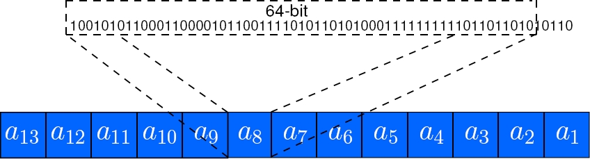
As it was mentioned in the Introduction, all the arithmetic operations are performed over a finite field
CPU servers have a 64-bit wordsize, we are forced to represent the field elements using an integer array of
2.2 Field Multiplication
Let
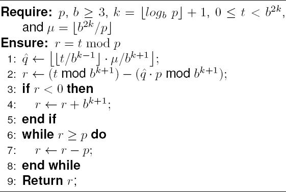
One can do better by using the Barrett reduction algorithm [5]. The Barrett reduction algorithm is based in the following observation: Given
For efficiency reasons, the method requires to precompute a per-modulus constant parameter:
where
Notice that upon finding
Algorithm 1 presents the Barrett reduction, where the remainder
2.3 Main Matrix-Vector Product Arithmetic Operations
The core arithmetic operation needed to perform a matrix-vector product is
For the set of matrices considered in this work, the coefficients
We took advantage of this fact (as shown in Fig. 2) by using the function row_multqu that starts a row-vector multiplication computing a field multiplication using the function Fp_mulC. The result of this function is stored in the accumulator
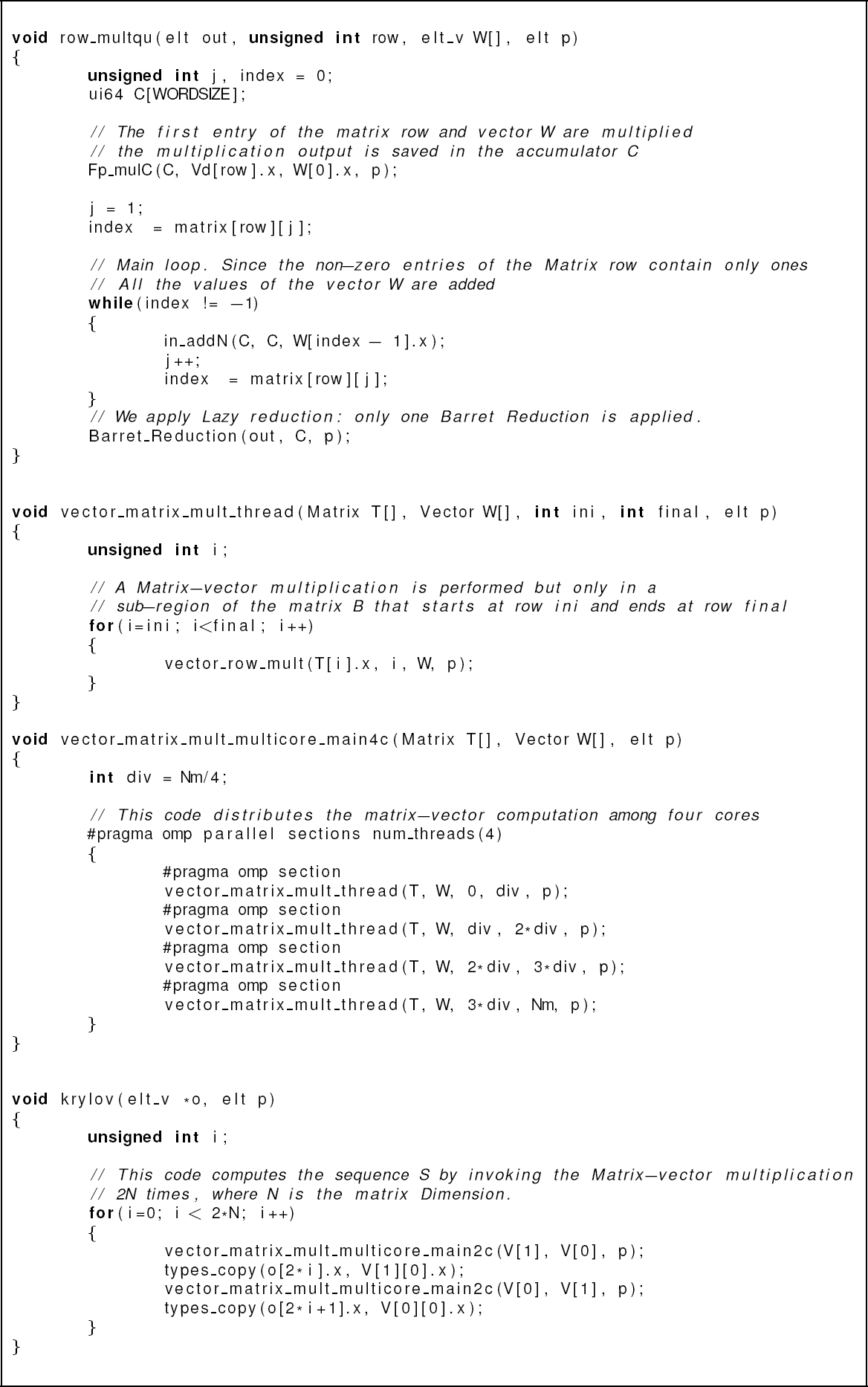
Taking advantage of the so-called lazy reduction technique, this addition function does not perform any modular reduction at all. Therefore, at the end of the function row_multqu’s loop, our Barret_Reduction function is invoked to guarantee that the final result (labelled as out) has an integer value into
For the families of matrices where
3 Wiedemann Algorithm
In this section, we describe our strategy for computing the kernel of thousands of sparse matrices.
We begin by describing the mathematics behind the Wiedemann algorithm and continue giving the main parallel strategies followed to compute the kernel of thousands of large sparse matrices.
We are targeting multi-core CPU servers, the super-computer ABACUS [7], and GPU Kepler architecture TITAN cards.
3.1 Basic Version of Wiedemann Algorithm
Let
Notice that each one of the coefficients in the sequence
is known as the minimum
The exponent
hence,
Therefore, in a third phase of Wiedemann algorithm, the minimum polynomial
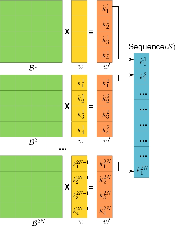
1. Krylov sequence: To obtain the Krylov sequence
Once again, the first coefficient of each one of the
2. Obtaining the minimum Polynomial
3. Minimum Polynomial Evaluation: It finds the solution
Hence, the computational cost of Wiedemann algorithm is dominated by phases 1 and 3, with an approximately overall cost of about
3.2 Exploiting Parallelism Opportunities in Wiedemann Algorithm
In 1994, Coppersmith famously presented a parallel version of Wiedemann algorithm [8]. The next few years, Kaltofen and Villard published in [18, 27], a comprehensive analysis of Coppersmith’s block version of this procedure. Arguably the first full implementation of this algorithm was reported by Kaltofen and Lobo in [19].
In a nutshell, Coppersmith idea was to simultaneously process
This setting has two advantages. Firstly, the total number of iterations is reduced from
Let us recall that for the main case study of this work, we are interested in computing the kernel of thousands of matrices that were obtained from the discrete logarithm problem attack over the finite field
Table 1 Hardware used for solving the linear algebra problems
| Platform | Nodes | Cores | Frequency (@ GHz) | Compiler |
| Pakal | 1 | 20 | 2.4 | gcc 4.8.2 |
| Abacus I | 318 | 8904 | 2.6 | gcc 4.8.3 |
| Titan | 1 | 2688 | 0.876 | CUDA assembly |
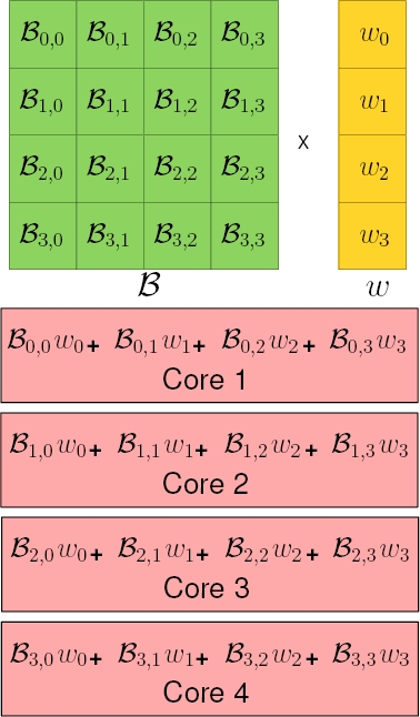
The matrix-vector product
Figure 4 depicts such partitioning for the case when four processing cores can be assigned to compute the kernel of a matrix
4 Implementation Aspects
Wiedemann algorithm was successfully implemented for computing the kernel of
To this end, we use the Pakal CPU server,3 the supercomputer ABACUS and a GPU Kepler architecture TITAN card, whose salient features are summarized in Table 1.
We begin this section by presenting the families of matrices considered in this work. Then, we give our theoretical cost estimates of computing the kernel associated to those matrices along with the real computational time obtained from our experiments.
4.1 Matrix Representation
In this work we only stored the non-zero values of a sparse matrix
For a comprehensive analysis of different techniques to store a sparse matrix, the interested reader is referred to [15, § 5.2].
4.2 Parallel Programming API
There exist several software tools for performing parallel computing, such as, Message Passing Interface (MPI), CUDA for GPU platforms, OpenMP, among others. In this work, we chose to use OpenMP [23] for our CPU server Pakal and the ABACUS supercomputer, and CUDA for our GPU Kepler architecture Titan card (refer to Table 1).
4.2.1 OpenMP for CPU Platforms
OpenMP defines a set of instructions for the C/C++ and Fortran programming languages, which makes easier to execute shared-memory parallelism.
A typical program using OpenMP instructions, starts with a single active master thread. Then, when the master thread execution reaches an OpenMP directive, such as the pragma directive omp parallel, it creates a set of threads specified by the programmer, where each of these threads will process a data set. Once that all the threads have performed their job, the master thread destroys the threads so created, and then it continues the sequential processing.
The segment that is processed in parallel depends on the given directive. For example, the directive sections divides the code into blocks and distributes each one of them among the participants threads. This directive is not sequential.
The parallel matrix-vector product strategy depicted in Figure 4, was implemented in C using OpenMP as reported in Appendix A. Indeed, the C coded function vector_matrix_mult_thread, performs a matrix-vector multiplication, but only in a sub-region of the matrix
4.2.2 CUDA for GPU Platforms
Graphic Processing Units (GPU), are massively parallel processors consisting of hundreds of cores. By taking advantage of the highly parallel architecture of the GPUs, one can speed up several computations where high computing power is required.
A typical GPU is composed by several processors. Each processor has a large number of cores, and each core execute threads. A GPU architecture groups the threads into blocks, and the blocks into a grid.
In the case of the implementation reported in this work, for each block we assign 32 threads to process 32 adjacent rows of the sparse matrix being handled. This process was repeated until all the columns of the matrix have been assigned. We implemented all the field arithmetic (addition, subtraction, multiplication and reduction) using CUDA assembly.4
4.3 Families of Matrices
We considered three different families of matrices. These matrices arise from the index-calculus method used in [2] to attack the discrete logarithm problem over the field
— Family of Quadratics: A single N-dimension sparse matrix with
— Family of Cubics:
— Family of Quartics:
Following the convention used in [2, 3], the first column of each one of the Cubics and Quartics matrices contains a large 804-bit non-zero entry. The salient features of these three systems are summarized in Table 2.
Table 2 Main features of the three families of linear algebra systems under study
| Quadratics | Cubics | Quartics | |
| Number of matrices | 1 | 728 | 21,141 |
| Dimension N | 266,086 | 177,391 |
|
| Per-row density of non-zero entries( |
1,086 –1,096 | 226 – 262 | 112 |
| number of nonzero entries |
|
|
|
From the characteristic of each matrix family, one can estimate the number of operations that a sequential execution would require for solving each linear algebra system.
4.3.1 Finding the Kernel of the Quadratics Matrix
Since the non-zero values of the Quadratics matrix are smaller than four, each scalar multiplication can be performed using a shift-and-add approach. As a first order approximation, let us assume that the cost of each one of these scalar multiplications is equivalent to one addition. Moreover, at the end of a row-vector multiplication, a Barrett reduction using Algorithm 1 is performed with an associated cost of at most two multiplications.
Then, the cost of a matrix-vector multiplication is of,
The Quadratics matrix was solved using our C implementation of Wiedemann’s algorithm; the computation took
4.3.2 Finding the Kernels of the Cubics Matrices
Since except for the first entry, the per-row non-zero values of the Cubics matrices are all equal to one, the cost of a row-vector multiplication is of
The 728 Cubics matrices were solved using our C implementation of Wiedemann’s algorithm. Each linear system was solved in parallel on 7 ABACUS cores. The 728 linear systems were solved simultaneously using 5096 ABACUS cores. The total execution time was
This time, and also the time for the linear algebra for the quartics (see §4.3.3), was more than expected in part because ABACUS was still running in an experimental phase and the machine was under-clocked to prevent over-heating. The increased CPU time did not have a significant impact on the total calendar time because of the large number of cores that we were at our disposal. The
Using seven cores per matrix, the elapsed time for the linear algebra computation of each one of the Cubics matrices was of about 74.4 hours. Significantly, the Titan implementation of this problem took only 24.3 hours by using
4.3.3 Finding the Kernels of the Quartics Matrices
Since except for the first entry, the per-row non-zero values of the Quartics matrices are all equal to one, the cost of a row-vector multiplication is of
Hence, the cost of a matrix-vector multiplication can be estimated in about
The
Using two cores per matrix, the elapsed time for the linear algebra computation of each one of the Quartics matrices was of about 19.62 hours. Significantly, the Titan implementation of this problem took only 0.96 hours by using
4.4 Comparison
Table 3 reports a comparison of the elapsed time required by our linear algebra solver CPU and GPU implementations. It is interesting to note that a GPU solution is remarkably faster than a CPU implementation for the case of the Cubics and Quartics families. However, the CPU implementation outperform its GPU counter part for the computation of the quadratics matrix.
Table 3 A comparison of the GPU and CPU elapsed time for computing the kernels of the three linear algebra system families
| Quadratics | Cubics | Quartics | |
| Matrix size( |
|||
| # Matrices | 1 | 728 | 21141 |
| Cores (CPU) | 20 | 7 | 2 |
| Threads (GPU) | 3584 | 3584 | 3584 |
| Linear Algebra CPU (hours) | 216 |
|
|
| Linear Algebra GPU (hours) | 223.2 |
|
|
| Speedup | - | 3.06 | 20.42 |
| MinPoly (hours) | 64.8 |
|
|
We believe that this behavior is due to the large size of this matrix that causes a costly divergence among the thread computations.
Due to the unique characteristics of the matrices derived in [2], it is in general difficult to compare our implementation with other related works. However, for the sake of completeness, we report in Table 4 a comparison of our GPU implementation against the one reported in [14]. The state-of-the-art software for computing Wiedemann algorithm is the CADO-NFS C implementation of the Number Field Sieve (NFS) algorithm for integer factorization and for computing discrete logarithms over finite fields [25]. However, we stress that the software in [25] specializes in the computation of usually one huge sparse matrix, but not in the simultaneous computation of thousands of large sparse matrices as is the case addressed in this work. Moreover, the GPU-based implementation of the CADO-NFS software basically corresponds to the work reported in [14], which is included in Table 4.
Table 4 A comparison of linear algebra solvers in GPU platforms
| Author | GPU | Matrix size | Modulus size | Timing (hours) |
| [14] | GeForce GTX 580 @1544MHz, 512 cores | 650K | 217 bits | 16 |
| This work | Titan, 2688 cores | 531K | 155 bits | 18.8 |
5 Conclusion
In this work, we reported the successful implementation of the null-spaces associated with
The CPU years associated with this task is summarized in Table 5, where the CPU frequency column lists the average clock speed of the cores used. In order to accomplish the solution of this task in a reasonable calendar time, we use several parallel and supercomputing techniques both, in CPU and GPU platforms.

