


Servicios Personalizados
Revista
Articulo
 texto en
  Inglés (pdf)
 Artículo en XML
 Referencias del artículo
 Enviar artículo por email
Indicadores
-
 Citado por SciELO
 -
 Accesos
Links relacionados
-
 Similares en
SciELO
Similares en
SciELO
Compartir

 Permalink
Problemas del desarrollo
versión impresa ISSN 0301-7036
Prob. Des vol.57 no.224 Ciudad de México ene./mar. 2026 Epub 22-Jun-2026
https://doi.org/10.22201/iiec.20078951e.2026.224.70429
Articles
Impact of welfare programs on income and corn production in Mexico
1 Benemérita Universidad Autónoma de Puebla (BUAP), México. Correo electrónico: pablo.corte@correo.buap.mx
This article aims to carry out an impact assessment of welfare programs targeting the Mexican countryside using the Kernel matching process. The hypothesis is that income and corn production are both significant for the beneficiaries of this policy. Statistical information from the National Household Income and Expenditure Survey and the 2022 Agricultural Census is used. The results demonstrate significant benefits in terms of income and corn production. Final reflections point out room for improvement in this policy.
Key words: impact assessment; average treatment effects; income; welfare programs; corn production
El objetivo de este artículo es realizar una evaluación de impacto de los programas del Bienestar dirigidos al campo mexicano utilizando el proceso de empa rejamiento de Kernel. La hipótesis sostiene que tanto los ingresos como la producción de maíz son significativos para los que son beneficiarios de esta política. Se utiliza la información estadística de la Encuesta Nacional de Ingreso y Gasto de los Hogares y del Censo Agropecuario 2022. Los resultados muestran que existen beneficios representa tivos tanto en ingresos como en producción de maíz. En las reflexiones finales se señala que se tienen condiciones para mejorar esta política.
Palabras clave: evaluación de impacto; efectos de tratamiento promedio; ingresos; programas del Bienestar; producción de maíz
Clasificación JEL: C21; C52; D19; I38; Q18
1. Introduction
At the beginning of Andrés Manuel López Obrador's six-year presidency (at the end of 2018), changes were made to the organizational structure of social policies. The countryside was no exception. The Direct Support Program for the Countryside (PROCAMPO) was established during the administration of Carlos Salinas de Gortari when the North American Free Trade Agreement (NAFTA) with the United States and Canada was about to take effect in 1994. This program aimed to support vulnerable rural households through financial transfers.
The López Obrador administration introduced a series of support measures known as the “Welfare Programs,” including the “Benito Juárez” scholarships, Youth Building the Future, Pensions for Elderly Men and Women and the Rita Cetina Universal Basic Education Scholarship, among others.
In the case of the countryside, these are the well-known programs: Guaranteed Prices, Sowing Life and Production for Welfare.
These programs seek to increase the income of their beneficiaries and improve production conditions in rural Mexico.
This study evaluates the effects of these rural welfare programs on corn producers in terms of income and production. It is also based on the hypothesis that the programs have a positive and significant impact.
Using information from the 2022 National Household Income and Expenditure Survey (ENIGH) (INEGI, 2023) and support from the Microdata Laboratory of the National Institute of Statistics and Geography (INEGI, 2023) for information from the Agricultural Census of the same year, the Kernel matching process was used to calculate the average treatment effects, measuring the different impacts on both beneficiaries and non-beneficiaries of the Welfare Programs.
In general, beneficiaries have higher incomes and greater corn production than “non-beneficiaries”.
The text is structured as follows: The second section reviews recent policies applied to the agricultural sector, covering the period from Carlos Salinas de Gortari to the present day, including an analysis of the evolution of corn production. The third section addresses the importance of conducting impact assessments using recent examples. The fourth section provides a methodological overview of kernel matching. The fifth section specifies the applied model and the sources of information. Section six shows the results obtained and, finally, section seven presents the conclusion.
2. Rural policy since the 1990s
At the beginning of 1992, a series of changes were made to Article 27 of the Political Constitution of the United Mexican States, which canceled agrarian distribution, while authorizing legal entities and other individuals with commercial exploitation interests to acquire agricultural land (Gómez de Silva Cano, 2016), thus bringing to an end policies based on protecting “ejidos.”
According to Alvarado Mendoza (1996), the intention behind opening up the agricultural sector to private parties was to enact legislative reforms prior to the NAFTA negotiations. One reason for this reform, according to the author, was that agricultural production already accounted for less than 10% of the GDP of Mexico.
To provide legal protection to both ejido landholders and private landowners regarding the possession of land, the Program for the Certification of Ejido Rights and Title to Urban Land was created to register agricultural land.
Simultaneously, PROCAMPO was established in 1993 to support a representative number of small producers vulnerable to market conditions. It remained in force for 20 years, changing its name to the Agricultural Development Program (PROAGRO) during the presidency of Enrique Peña Nieto. These policies, along with the National Solidarity Program (PRONASOL), aimed to alleviate the inherent poverty in rural areas caused by commercial competition with products from the United States and Canada (Gutiérrez Espinosa and Rabell García, 2018).
However, although agricultural production in Mexico had been declining since the mid-1960s, the implementation of the reforms did not have the desired effect of increasing production and, with the arrival of the North American Free Trade Agreement, it was unable to reverse the decline in growth rates, causing the sector to contract further until 2013 (Escalante Semerena and González, 2018).
According to Hernández Pérez (2021), the implemented reforms led to changes in the production structure, reducing the number of hectares dedicated to farming compared to 1995. According to the author, this has increased food dependency; however, since 2014, agricultural exports have slightly exceeded imports. Hernández Pérez also points out that this model has led to higher unemployment in the sector.
It should be noted that agricultural production had already been declining since the mid-1970s, as the economy focused on industry and trade, dispelling the idea that the primary sector was the basis of the economy and its development. Although attempts were made to rescue the rural sector during that decade, the other sectors consolidated the trend. By the end of the 1980s, the ideal of agriculture being a fundamental part of the national economy was unrealistic (Grammont, 2010). Indeed, Salinas Calleja (2004) highlighted the decline in the dynamism of the sector, as its growth rate fell from 4.2% in the 1970s to 0.5% in the 1980s.
At the time of the reform, the share of the primary sector accounted for less than 4% of the total economy and, between 1993 and 2025, this level remained at around 3%, according to INEGI data (2025), which also shows that, despite the favorable outlook for other economic sectors, there are avenues for dynamism in agricultural production.
In view of the above, all these programs have been described as welfare-oriented, as they consist solely of financial transfers that enable low-income populations to increase their consumption without altering their original economic status (Márquez Covarrubias, 2022).
In response to this, social policy has taken a new direction, aiming to combat poverty and also to promote productivity in various areas. One example is the Youth Building the Future program, which provides young people with access to paid employment through training and monthly scholarships of up to MXN$8,480.17 (Ministry of Labor and Social Welfare, 2025).
Considering the development of rural areas, three programs were established at the start of the six-year presidency of Andrés Manuel López Obrador: Guaranteed Prices, Sowing Life and Production for Welfare (the latter is a continuation of PROCAMPO/PROAGRO).
The Guaranteed Price Program aims to help grain and milk producers supplement their income and increase their production. In the case of corn, a price of MXN$5,840.00 per ton was established, depending on the agricultural cycle and provided it does not exceed 35 tons, according to the Official Gazette of the Federation (DOF, January 30, 2025).
The Sowing Life program supports rural residents in municipalities with high levels of social deprivation who own no more than 2.5 hectares by providing monthly financial transfers of MXN$6,500.00, in-kind assistance and technical support (DOF, February 21, 2025).
The third program, Production for Welfare, focuses on providing financial support to small- and medium-scale producers (up to 20 hectares for rainfed crops and five hectares for irrigated crops) of products such as corn, wheat, beans, rice, amaranth, sugarcane, coffee, nopal, cacao and honey, among others. Many of these producers already received support from previous programs. Annual payments range from MXN$6,400.00 to MXN$10,000.00 depending on the product and the size of the property on which it is grown (DOF, January 28, 2025).
Regarding these programs, De Ita (2018) notes:
It is a way of boosting the regional economy and rural production by supporting them with payments for rural work [...] producers will be guaranteed different harvested products. Agricultural productivity is expected to increase, while the increase in family income will help to contain migration (p. 59).
When examining these rural programs, it is essential that we review corn production. It should be noted that corn was selected because it forms the basis of the Mexican (and Mesoamerican) diet in addition to being the most representative crop, given that it is the staple ingredient in tortillas, tamales and other consumer items. Geographically speaking, corn is well suited for planting and harvesting due to its adaptability to different climates, which is why, in economic terms, it represents the country's most important agricultural value chain.
The aforementioned policies obviously affect the production of this commodity, so it is important to analyze its evolution from 1980 to 2023 (see Figure 1).
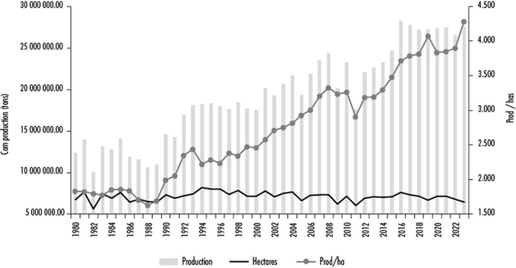
Source: Prepared by the author using data from the Agrifood and Fisheries System (SIAP, undated). https://nube.agricultura.gob.mx/cierre_agricola/
Figure 1 Evolution of corn production 1980-2023
From 1980 until the agrarian reform of 1992, productivity per hectare grew at an average annual rate of 2.1% while, from 1992 until the end of Ernesto Zedillo's presidency, productivity grew at a rate of only 0.6%, possibly due to the 1995-1996 recession.
Despite the decline in corn production in 2011, the PAN era (2000-2012) saw an average annual growth rate of nearly 2.2%, while in the 2012-2018 presidential term, corn production per hectare grew by 3% annually.
Clearly, while corn production has increased, the number of hectares has decreased between 1980 and 2023. Thus, this increase in productivity may be due to various factors. Some authors, such as Favila Tello and Reyes Ponce (2022), have examined this behavior and it is worth taking a closer look at what they have to say about it.
Ayala-Garay and Hernández Vásquez (2024) point out differences in production processes: some are large-scale, some are small-scale and some conventional processes, while others use agroecological practices. These distinctions are useful for interpreting the information on how medium- and large-scale producers may be better represented, which obscures the actions of small producers in official statistics (see Figure 1).
Grammont (2010) offers a clear explanation for this behavior, indicating that the reforms carried out in 1992 divided the countryside into two coexisting polarized areas. First, promotion of public policy in the sector was abandoned so that small and large production units would not enter the market. Second, contract farming was introduced to strengthen value chains, leading to a process of capitalization despite fewer agricultural households and increased technology in the sector.
3. Impact assessment and its importance in evaluating public programs
Different public bodies implement policies aimed at addressing specific issues such as educational disadvantages, job training, health, improved income, increased production in underdeveloped communities, etc. In accordance with the National Council for the Evaluation of the Social Development Policy (CONEVAL, 2023), governments implement policies that seek to reduce the negative impacts caused by drought, unemployment, malnutrition, poverty and other factors affecting the community.
For this reason, we need to evaluate the social programs that have been implemented to determine how well they are working and improve them if necessary (Corte Cruz, 2024). This requires identifying two key groups: the treatment group, who are beneficiaries of the program and the control group, who are not.
Impact assessments have been carried out in various areas where social policies have been implemented, including education, health and poverty alleviation. Rawlings and Rubio (2003) conducted assessments in these sectors in various regions of Latin America using the Propensity Score Matching (PSM) method and their results show that, regarding education, countries that implement financial transfers, such as Nicaragua, Brazil and Mexico, increase school enrollment and reduce child labor. In terms of health, they increase the use of clinical and hospital services, reducing maternal and infant mortality.
The Difference-in-Difference method has also been applied in education to analyze the Full-Time Schools program implemented during the governments of Felipe Calderón (2006-2012) and Peña Nieto (2012-2018). This program was found to have positive effects on academic performance, particularly in Spanish, resulting in an average increase of 25.64 points on tests for this subject. However, although the results in mathematics were also positive, they did not reach statistical significance (Luna Bazaldúa and Velázquez Villa, 2019).
Another analysis of fighting poverty through income is that of Cecchiniet al.(2021), based on a comparison of poverty levels in 15 Latin American countries between 2014 and 2017. They demonstrate that financial transfer programs have succeeded in reducing poverty and, more importantly, precarious conditions by between 0.4 and 11.9%.
Boruchowicz (2019) evaluated the Urban Integration and Coexistence Program launched in Honduras, in which, when applying a PSM, the only significant result for the beneficiaries of this policy was in the service sector regarding sewerage connections, while there were no statistically significant consequences in other areas.
Regarding social programs for rural areas, González Flores and Le Pommellec (2019) employed the Differences-in-Differences and PSM methods in a study of the Environmental Program for Disaster Risk Management and Climate Change (PAGRICC), which was implemented in Nicaragua. They found that, first, there is indeed an increase in agricultural production measured per hectare and that the beneficiaries of the program are more resilient to the harmful effects of climate change.
Meanwhile, Silva Vargas (2021) used the PSM to calculate the average treatment effect (ATE) and the average treatment effect on the treated group (ATT) in an evaluation of the PROCAMPO program for bean production. She noted that beneficiaries expanded the number of hectares for this crop and increased its production in 2008.
Focusing specifically on welfare programs aimed at the rural sector, using a qualitative methodology, CONEVAL (2024) analyzed the effectiveness of the Sembrando Vida (Sowing Life) policy in four key areas: food security, economic welfare, the sustainability of agroforestry systems and the strengthening of the social fabric. The results indicate that both food availability and nutrition improved, rural household income increased and progress was made in the acquisition of bio-inputs and the adoption of native seeds, generating greater social cohesion in rural areas.
While there are more examples of evaluations carried out, it should also be noted that there are different contexts, including for each program, so results may vary, depending mainly on the methodology used.
4. The Kernel matching method
This study seeks to determine the effects of the treatment group compared to what would have happened if they had not received support from the program. The presence of selection bias must be considered because beneficiaries enroll voluntarily. In the absence of randomization, we must identify whether this represents a conflict for the evaluation process.
To measure the effects, the ATE, ATT and average treatment effect on the control group (ATC) are calculated:
In this case, X is the vector of explanatory variables with respect to income and production (as applicable) and Z is the vector of independent variables with respect to the variable that determines whether or not someone receives support from the welfare program.
Matching techniques are based on observing similarities between the treatment and control groups, so the Kernel method relies on comparing them by minimizing the characteristic distance or the properties of the estimators that allow for such an evaluation (Aedo, 2005, cited in Ferrada and Montaña, 2022).
An important part of this method is calculating a PSM based on alogitmodel, which, by using a density function, reviews the distribution of both the treatment and control groups. This measurement is generated through:
Two elements are constructed from the PSM. The first is the common support zone (ZSC), which compares the treatment group (T = 1) with the control group (T = 0), determining all those who statistically have the same conditions and are eligible to receive support from the social program under review. The second element is the calculation of the distance of properties proposed by Prasanta Chandra Mahalanobis (Escobedo Portillo and Salas Plata Mendoza, 2008), which validates both sides of the study, i.e. the treatment and control groups.
The Kernel Matching method considers the influence of variables affecting the direct counterpart of the evaluation, using ordinary least squares (OLS). Instead of considering an exogenous response, it considers an endogenous one because there are variables on which they also depend (Cameron and Trivedi, 2005).
These elements form the basis for conducting the impact assessment through the aforementioned average treatment effects using the Kernel Matching method:
Establishing β and γ as vectors of the parametric values of the OLS andlogitregressions, respectively.
Prior to this operation, we must analyze whether selection bias could cause statistical errors in the evaluation process, which could invalidate the process. For this reason, we must perform a Heckman regression to calculate the Inverse Mills Ratio (IMR). The aim is to determine whether (or not) this situation could distort the desired results (Martín-Conejero and Quirós-González, 2024).
It should be noted that selection bias always exists because participation is voluntary, not random.
Values (4) and (5) are required to carry this out, unless aprobitregression is used instead of alogitregression:
where Φ is the standard normal cumulative distribution function and σ is the parameter vector of theprobitregression.
The IMR is then calculated by dividing the standard normal probability density function evaluated in the results of theprobitregression by the standard normal cumulative distribution function:
If λ (i.e., the IMR) is statistically significant, selection bias could cause statistical problems; otherwise, the assessment may be accurate.
The Kernel Matching method uses the Mahalanobis distance to find individuals in the control group who resemble those in the treatment group based on the same characteristics. This reduces selection bias and seeks to correct for it, which is one of the advantages of this method. Another reason for using the Kernel Matching method is that it can be specified that this matching be carried out for each federal state.
5. Model and sources of information
The first step is to conduct OLS regressions to analyze the behavior of income and production. In the first case, given the availability of information from the 2022 ENIGH survey (INEGI, 2023), the following model is established:
whereagerefers to the age of the household head,ethnicityrefers to whether said head identifies as indigenous or Afro-descendant,hworkrepresents hours worked and yearsstud represents the average years of study in the household. This model is based on the proposal by Godínez Montoyaet al.(2015), who analyzed the dependent variable in some areas of the state of Chiapas. Age-squared (age2) is based on Franco Modigliani's model, which states that when people reach a certain age, they retire and their income decreases.
In the case of corn production, the nature of the information required permission from the INEGI Microdata Laboratory to access the 2022 Agricultural Census. Data from this census was used to develop a Cobb-Douglas model:
where the initial letterlrefers to working with the logarithm of corn production (prod), hectares (land), number of workers (work) and physical capital (capital).
Thelogitmodels for income and corn production, are based on Pucutay Vázquez (2002), where age, household size (rooms), the sex of the household head (sexheadhouse), belonging to an indigenous or Afro-descendant group (ethnicity) and receiving other benefits (e.g., support for the elderly (AAM)) influence individual decisions to receive public policy benefits.
In the case of income, thelogitfunction ofwelfareis established as follows:
In the case of corn production, thelogitfunction is:
Thewelfarevariable is binary, where 1 refers to households and productive units that receive at least one of the three rural welfare programs. The models do not converge due to the characteristics and nature of how both the ENIGH and the Agricultural Census were conducted.
Based on equations (3) and (4), the ZSCs where both the treatment and control groups are located can be determined for income and corn production.
To verify whether selection bias can generate evaluation conflicts, a James Heckman regression is performed to calculate the IMR, which is the result of equation (8).
Kernel Matching regression is applied using (9) and (11) for income and (10) and (12) for production to calculate the treatment effects (1), (2) and (3) for each case, in order to subsequently verify whether the selection bias is corrected in the post-estimation process.
6. Results
Regarding the results of the OLS for income, it should be clarified that the variables had to be transformed due to evidence of heteroscedasticity in order to perform the weighted OLS (see Table 1). Based on the results, the age2 variable is not statistically significant. Another notable variable isethnicity, which, despite the discourse of prioritizing indigenous and Afro-descendant populations, is negative. This means that these population groups have lower incomes, even in rural areas. Although the R-squared is too low, the ANOVA test indicates that joint statistical significance exists (see Table 1A).
Table 1 OLS regressions for income
| Dependent variable: income | |
|---|---|
| age | 412.9135** |
| (209.780) | |
| [1.97] | |
| age2 | -3.18 |
| (2.504) | |
| [-1.27] | |
| athnicity | -10 931.95* |
| (3 890.209) | |
| [-2.81] | |
| hwork | 588.1791* |
| (96.322) | |
| [6.11] | |
| yearsstud | 1 366.81* |
| (462.298) | |
| [2.96] | |
| R2 | 0.04 |
| Observations | 5 231.00 |
Notes: ( ) Standard error; [ ] t-statistic. * Significance level of 0.01; ** significance level of 0.05; *** significance level of 0.10.
Source: Prepared by the autor using STATA 16 with data from the 2022 ENIGH, https://www.inegi.org.mx/programas/enigh/nc/2022/
Table 1A ANOVA table for least squares regression on income
| Sources of variation | Sum of squares | Degrees of freedom | Average square | F | p-value |
|---|---|---|---|---|---|
| Regression | 2.45E+12 | 5 | 4.91E+11 | 45.61 | 0.0000 |
| Error | 5.62E+13 | 5 226 | 1.08E+10 | ||
| Total | 5.87E+13 | 5 231 |
Source: Prepared by the author using STATA 16 based on the information provided by the regression in Table 1.
The results in Table 2 indicate that the work variable is not statistically significant. Nevertheless, it was decided to keep it in the model because labor is an essential component of agricultural production. It should be noted that physical capital is negative and significant. As in Table 1, the goodness-of-fit statistic (R2) is very low, suggesting that the included variables only explain a limited portion of the variability in corn production. Despite this, the ANOVA table (see Table 2A) shows overall significance, meaning that each regressor element significantly contributes to explaining the regressed variable.
Table 2 OLS regression for corn production
| independent variable: logarithm of corn production | |
|---|---|
| Land logarithm | 0.1620* |
| (0.001) | |
| [164.20] | |
| Work logarithm | 0.0004 |
| (0.002) | |
| [.26] | |
| Physical capital logarithm | -1.8319* |
| (0.005) | |
| [-348.32] | |
| Constant | 1.3923* |
| (0.004) | |
| [338.98] | |
| R2 | 0.0929 |
| Observations | 1440674 |
Notes: ( ) standard error; [ ] t-statistic; * significance level of 0.01; ** significance level of 0.05; *** significance level of 0.10.
Source: Prepared by the author in the Microdata Laboratory using information from the 2022 Agricultural Census.
Table 2A ANOVA of the least squares regression on corn production
| Sources of variation | Sum of squares | Degrees of freedom | Average square | F | p-value |
|---|---|---|---|---|---|
| Regression | 4.56E+05 | 3 | 1.52E+05 | 49 194.58 | 0.0000 |
| Error | 4.45E+06 | 1 440 670 | 3.09E+00 | ||
| Total | 4.91E+06 | 1 440 673 |
Source: Prepared by the autor base don information from the regression inTable 2.
In thelogitregression process set out in equations (3) and (4), older age and belonging to an ethnic group (or being of African descent) are considered to increase the probability of receiving support from welfare programs. Likewise, having a larger home or receiving support for reasons other than living in the countryside (e.g., support given to the elderly) reduces the likelihood of being covered by this policy. Notably, households headed by women have fewer opportunities to receive the aforementioned social programs (see Table 3).
Table 3 Logit regression OF Welfare for income and production
| Dependent variable: Welfare | ||
|---|---|---|
| Variables | Income | Production |
| Age | 0.0090* | 0.0416* |
| (0.002) | (0.000) | |
| [4.60] | [435.14] | |
| Ethnicity | 0.1560* | 0.4810* |
| (0.058) | (0.003) | |
| [2.69] | [168.11] | |
| Rooms | -0.0514* | |
| ´(0.019) | ||
| [-2.69] | ||
| Sex household head | -0.4778* | |
| (0.098) | ||
| [-4.85] | ||
| Support for the elderlyr | -0.3318* | |
| (0.004) | ||
| [-79.74] | ||
| Constant | -0.5690* | -2.9455* |
| (0.137) | (0.005) | |
| [-4.16] | [-606.28] | |
| Pseudo R2 | 0.0076 | 0.1344 |
| LR chi2 | 54.69 | 45 050.7 |
| P-Value(chi2) | 0.0000 | 0.0000 |
| Observations | 5 231 | 2 678 288 |
Notes: ( ) standard error; [ ] t-statistic; * significance level of 0.01; ** significance level of 0.05; *** significance level of 0.10.
Source: Prepared by the autor using STATA with information from the ENIGH and the Microdata Laboratory for the 2022 Agricultural Census.
Analyzing the ZSCs (see Figure 2) for both income and corn production reveals the population groups included in the evaluation. These groups consist of those who are eligible for support as opposed to those who are not eligible but have similar statistical characteristics.
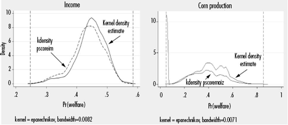
Source: Prepared by the author using STATA with information from ENIGH and the Microdata Laboratory for the 2022 Agricultural Census.
Figure 2 Common support zones
Regarding income, the matching group below the solid and dotted lines appears to be well-defined. In the case of production, the line initially has a high density and is established immediately below the curve representing the treatment group. The population groups with which matching is carried out are already established (see Figure 2).
Prior to the evaluation, the Heckman regression is performed to verify whether the presence of selection bias could be a statistical problem. This regression is based on OLS regressions (9) and (10), as well as (11) and (12) in theirprobitversion (see results in Table 4).
Tabla 4 Resultado de la IMR a partir de la regresión de Heckman
| Income | Production | |
|---|---|---|
| IMR | -0.0381 | 0.4232 |
| Standard error | 0.845 | 0.003 |
| p-value | 0.9640 | 0.0000 |
Source: Prepared by the autor base don results obtained from ENIGH data and data provided by the Microdata Laboratory for the 2022 Agricultural Census.
In terms of income, it is shown that selection bias may not be a statistical conflict for the evaluation process, while in terms of production, the aim is to correct this situation using the Kernel Matching process. As previously mentioned, the Mahalanobis statistical distance involves searching for a more accurate match, verifying these results for each federal state.
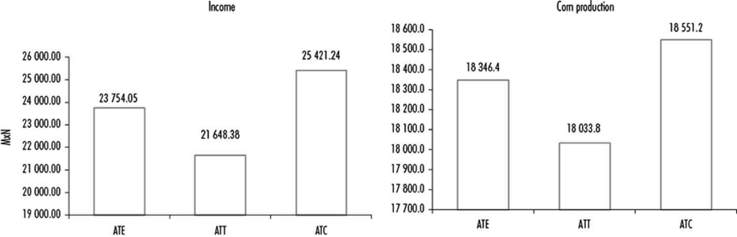
Based on these results, Figure 3 presents the average treatment effects calculated for both income and production using equation (6).
Source: Prepared by the author based on results obtained from ENIGH data and data provided by the Microdata Laboratory for the 2022 Agricultural Census.
Figure 3 Effects of average treatment on income and corn production
In the case of income from corn-producing households, beneficiaries received MxN$21,648.38 in current terms that year, indicating an increase in this category compared to if they were not enrolled in the programs. Note that if the control group received welfare support, they would receive MXN$25,421.24. If both groups received the support, the ATE would be MXN$23,754.05 based on this policy.
In contrast, in the case of corn production, it should be noted that the average group size is nine hectares, i.e. they are small- and medium-sized producers, with the small-sized predominating. Therefore, the values established are per kilogram (kg), i.e. people receiving support from rural welfare programs produce just over 18,033 kg of corn compared to if they did not receive said support, while non-beneficiaries could produce 18,551.2 kg if enrolled in the program. If both groups received support, they would produce an average of 18,346.4 kg more. Note that both income and production results are annual.
To verify that these results are correct, one must check whether the Kernel matching method effectively corrected the selection bias (see Figure 4).
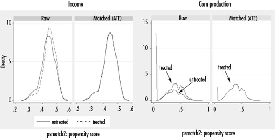
Source: Prepared by the author using STATA based on results obtained from ENIGH data and data provided by the Microdata Laboratory for the 2022 Agricultural Census.
Figure 4 Correction for selection bias
Based on the information regarding the correction of selection bias, it can be said that the aforementioned results are reliable, clearly establishing the effectiveness of social programs.
7. Conclusion
The impact assessment measures the effect of social programs by highlighting the difference in results obtained by beneficiaries compared to what they would have achieved if they had not been enrolled in the policy implemented for this purpose, thus identifying which areas work and which do not.
An impact assessment provides evidence of the effectiveness of public policies and informs decisions about whether to continue, improve and expand them if possible or to change course if they are not delivering the expected results. Finally, in the present case, the importance of public policies also lies in identifying the areas (income, production or both) in which they are effective.
This evaluation uses the kernel matching method, which, based on non-linear parameters, provides more robust results by reducing selection biases when comparing the control group with the treatment group based on similar statistical properties, thus achieving a more accurate match given the available information for the model.
While we could discuss how the evaluated program functions, two things must be considered: first, the sources of information. In this case, the ENIGH is used since INEGI has publicly available detailed information that facilitates the work. Conversely, in the case of the Agricultural Census, the information may be mishandled due to its nature so the Microdata Laboratory at the Institute must be used. This requires careful attention at every step, so the results must be adapted to the study carried out in this document.
The results of the OLS andlogitregressions show that individuals who identify as belonging to an ethnic group earn less income than the rest of the observed population but are more likely to receive welfare support. In contrast, female-headed households are less likely to receive support from the social program under study, which is notable.
Regarding income, we can see that welfare programs benefit corn-producing households each year, with average annual amounts exceeding $21,000 Mexican pesos (MXN), while the production for units producing this commodity exceeds 18,000 kg (18 tons). Although this amount seems lower, it should be noted that the maximum supported level is 20 hectares, which represents positive support for production.
Statistically, in the case of production, there is an initial bias that could affect the evaluation process. However, the Kernel Matching method uses Mahalanobis distance to correct for this bias by seeking conditions of statistical and spatial proximity, taking into account the characteristics of each federal state. Thus, the quantitative results shown are reliable.
Therefore, the average treatment effects shown in this analysis indicate that there are statistically significant advantages for both income and corn production, which means that the group of beneficiaries of welfare programs needs to be expanded because they are yielding significant results in favor of the treatment group.
Bibliografía
Aedo, C. (2005). Evaluación de Impacto. Serie Manuales CEPAL. 47. https://repositorio.cepal.org/server/api/core/bitstreams/a32d735a-3408-4ff8-9216-af2ccb05cf47/content [ Links ]
Alvarado Mendoza, A. (1996). Entre la reforma y la rebelión: el campo durante el salinismo. Foro Internacional, 36(1). https://repositorio.colmex.mx/concern/articles/xs55mc68r [ Links ]
Ayala-Garay, A. V. y Hernández-Vásquez, B. (2024). Rentabilidad de la producción de maíz en sistemas agroecológico y convencional en dos comunidades de Tlaxcala. Agricultura, Sociedad y Desarrollo. 21(1). https://doi.org/10.22231/asyd.v21i1.1566 [ Links ]
Boruchowicz, C. (2019). Programa de Integración y Convivencia Urbana: Resultados de la Estrategia de Pareamiento. (Documento para Discusión NO IDB-DP-00636). Sector de Cambio Climático y Desarrollo Sostenible, División de Vivienda y Desarrollo Urbano, Banco Interamericano de Desarrollo. https://publications.iadb.org/es/programa-de-integracion-y-convivencia-urbana-resultados-de-la-estrategia-de-pareamiento-dataset [ Links ]
Cameron, C. y Trivedi, P. (2005). Microeconometrics. Methods and applications. Cambridge University Press. [ Links ]
Cecchini, S., Villatoro, P. y Mancero, X. (2021). El impacto de las transferencias monetarias no contributivas sobre la pobreza en América Latina. Comisión Económica para América Latina y el Caribe (CEPAL). https://repositorio.cepal.org/server/api/core/bitstreams/25b6a515-182d-4a7d-8f68-87443adbaee9/content [ Links ]
Consejo Nacional de Evaluación de la Política de Desarrollo Social (CONEVAL) (2023). Informe de Evaluación de la Política de Desarrollo Social 2022. CONEVAL https://www.coneval.org.mx/EvaluacionDS/PP/CEIPP/Documents/Informes/IEPDS_2022.pdf [ Links ]
______ (2024). Evaluación de Impacto Cualitativo del Programa Sembrando Vida. CONEVAL. https://www.coneval.org.mx/EvaluacionDS/PP/CEIPP/Documents/EVALUACIONES/Evaluacion_impacto_PSV/Evaluacion_de_impacto_PSV.pdf [ Links ]
Corte Cruz, P. S. (2024). Evaluación de impacto a los programas PROAGRO y Bienestar sobre los ingresos en los hogares rurales en la región Golfo-Centro de México. Revista de Economía, 41(103). https://doi.org/10.33937/reveco.2024.409 [ Links ]
De Ita, A. (2018). AMLO: claroscuros de propuestas para el campo. El Cotidiano, 213. https://ceccam.org/sites/default/files/AMLOclaroscuros.pdf [ Links ]
Diario Oficial de la Federación (DOF) (2025, 28 de enero). Acuerdo por el que se dan a conocer las Reglas de Operación del Programa Producción para el Bienestar de la Secretaría de Agricultura y Desarrollo Rural para el ejercicio fiscal 2025. https://www.dof.gob.mx/nota_detalle.php?codigo=5747876&fecha=28/01/2025#gsc.tab=0 [ Links ]
______ (2025, 30 de enero). Acuerdo por el que se dan a conocer las Reglas de Operación del Programa de Precios de Garantía a Productos Alimentarios Básicos para el ejercicio fiscal 2025. https://dof.gob.mx/nota_detalle.php?codigo=5748189&fecha=30/01/2025#gsc.tab=0 [ Links ]
______ (2025, 21 de febrero). Acuerdo por el que se emiten las Reglas de Operación del Programa Sembrando Vida, para el ejercicio fiscal 2025. https://dof.gob.mx/nota_detalle.php?codigo=5749915&fecha=21/02/2025#gsc.tab=0 [ Links ]
Escalante Semerena, R. y González, F. (2018). El TLCAN en la agricultura de México: 23 años de malos tratos. Ola Financiera, 11(29). http://dx.doi.org/10.22201/fe.18701442.2018.29.64143 [ Links ]
Escobedo Portillo, M. T. y Salas Plata Mendoza, J. A. (2008). P. Ch. Mahalanobis y las aplicaciones de su distancia estadística. Cultura, Ciencia y Tecnología, 5(27). https://erevistas.uacj.mx/ojs/index.php/culcyt/article/view/385 [ Links ]
Favila Tello, A. y Reyes Ponce, Á. D. (2022). Indicadores de competitividad del maíz mexicano en el mercado de Estados Unidos. RECAI. Revista de Estudios en Contaduría, Administración e Informática, 11(32). https://doi.org/10.36677/recai.v11i32.19576 [ Links ]
Ferrada, L. M. y Montaña, V. (2022). Inclusión y alfabetización financiera: el caso de trabajadores estudiantes de nivel superior en Los Lagos, Chile. Estudios Gerenciales, 38(163). https://doi.org/10.18046/j.estger.2022.163.4949 [ Links ]
Godínez Montoya, L., Figueroa Hernández, E. y Pérez Soto, F. (2015). Determinantes del Ingreso en los Hogares en Zonas Rurales en Chiapas. Nóesis, 24(47). http://dx.doi.org/10.20983/noesis.2015.1.5 [ Links ]
Gómez de Silva Cano, J. J. (2016). El derecho agrario mexicano y la Constitución de 1917. Instituto Nacional de Estudios Históricos de las Revoluciones de México, Instituto de Investigaciones Jurídicas (UNAM). [ Links ]
González Flores, M. y Le Pommellec, M. (2019). Evaluación de Impacto del Componente 1 del Programa Ambiental de Gestión de Riesgos de Desastres y Cambio Climático (PAGRICC). (Nota técnica del BID, 1670). Banco Interamericano de Desarrollo. https://publications.iadb.org/es/evaluacion-de-impacto-del-componente-1-del-programa-ambiental-de-gestion-de-riesgos-de-desastres-y [ Links ]
Grammont, H. C. (2010). La evolución de la producción agropecuaria en el campo mexicano: concentración productiva, pobreza y pluriactividad. Andamios, 7(13). https://www.scielo.org.mx/pdf/anda/v7n13/v7n13a5.pdf [ Links ]
Gutiérrez Espinosa, D. J. y Rabell García, E. (2018). La política social en el campo mexicano. Misión Jurídica, 11(15). https://www.revistamisionjuridica.com/la-politica-social-en-el-campo-mexicano/ [ Links ]
Hernández Pérez, J. L. (2021). La agricultura mexicana del TLCAN al TMEC: consideraciones teóricas, balance general y perspectivas de desarrollo. El Trimestre Económico, 88(352). https://doi.org/10.20430/ete.v88i352.1274 [ Links ]
Instituto Nacional de Estadística y Geografía (INEGI) (2023). Encuesta Nacional de Ingreso y Gasto de los Hogares. https://www.inegi.org.mx/programas/enigh/nc/2022/ [ Links ]
______ (2025). Economía y Sectores Productivos. Agricultura. https://www.inegi.org.mx/temas/agricultura/ [ Links ]
Laboratorio de Microdatos (2023). Censo Agropecuario 2022. Instituto Nacional de Estadística y Geografía (INEGI). https://www.inegi.org.mx/microdatos/ [ Links ]
Luna Bazaldúa, D. A. y Velázquez Villa, P. G. (2019). Evaluación del impacto del Programa de Escuelas de Tiempo Completo en medidas de logro académico de centros escolares en México. Revista Latinoamericana de Estudios Educativos, 49(2). https://rlee.ibero.mx/index.php/rlee/article/view/19 [ Links ]
Márquez Covarrubias, H. (2022). Asistencialismo estatal: variantes de sujeción de los desposeídos. Observatorio del Desarrollo, 11(32). https://estudiosdeldesarrollo.mx/observatoriodeldesarrollo/numero-32/ [ Links ]
Martín-Conejero, A. y Quirós-González, V. (2024). Errores metodológicos. Sesgos. Angiología, 76(4). https://dx.doi.org/10.20960/angiologia.00665 [ Links ]
Pucutay Vázquez, F. (2002). Los modelos logit y probit en la investigación social. El caso de la pobreza del Perú en el año 2001. Centro de Investigación y Desarrollo del Instituto Nacional de Estadística e Informática (INEI), https://www.inei.gob.pe/media/MenuRecursivo/publicaciones_digitales/Est/Lib0515/Libro.pdf [ Links ]
Rawlings, L. B. y Rubio, G. M. (2003). Evaluación del impacto de los programas de transferencias condicionadas en efectivo: lecciones desde América Latina. (Cuadernos de Desarrollo Humano, No. 10). Secretaría de Desarrollo Social. http://www.oda-alc.org/documentos/1340861380.pdf [ Links ]
Salinas Calleja, E. (2004). Balance general del campo mexicano 1988-2002. El Cotidiano, 19(124). https://www.redalyc.org/pdf/325/32512401.pdf [ Links ]
Secretaría del Trabajo y Previsión Social (2025). Jóvenes construyendo el futuro. https://jovenesconstruyendoelfuturo.stps.gob.mx/ [ Links ]
Servicio de Información Agroalimentaria y Pesquera (SIAP) (s/f). Anuario Estadístico de la Producción Agrícola. https://nube.agricultura.gob.mx/cierre_agricola/ [ Links ]
Silva Vargas, Z. Y. (2021). Evaluación de impacto del Programa de Apoyos Directos al Campo sobre la producción de frijol en México en el año 2008. [Tesis de maestría]. Facultad Latinoamericana de Ciencias Sociales, Sede Académica de México. https://flacso.repositorioinstitucional.mx/jspui/bitstream/1026/376/1/Silva_ZY.pdf [ Links ]
Received: May 14, 2025; Accepted: October 31, 2025
 Este es un artículo publicado en acceso abierto bajo una licencia Creative Commons
