


Servicios Personalizados
Revista
Articulo
 texto en
  Inglés (pdf)
 Artículo en XML
 Referencias del artículo
 Enviar artículo por email
Indicadores
-
 Citado por SciELO
 -
 Accesos
Links relacionados
-
 Similares en
SciELO
Similares en
SciELO
Compartir

 Permalink
Problemas del desarrollo
versión impresa ISSN 0301-7036
Prob. Des vol.55 no.217 Ciudad de México abr./jun. 2024 Epub 18-Nov-2024
https://doi.org/10.22201/iiec.20078951e.2024.217.70116
Articles
Macroeconomics and poverty: an empirical review for Mexico 2005-2022
aUniversidad Nacional Autónoma de México (UNAM)-Facultad de Economía, México. Correo electrónico: marcomcal@economia.unam.mx
bConsejo Nacional de Evaluación de la Política de Desarrollo Social (CONEVAL) y UNAM-Instituto de Investigaciones Económicas, México. Correo electrónico: jnabor@unam.mx.
The article analyzes the relationship between macroeconomics and (labor) poverty between 2005 and 2022. Three scenarios were considered: 1) income, inflation, interest rate and labor poverty, while scenarios 2) and 3) considered labor income and inflation of lines of poverty and extreme poverty in relation to income, respectively. An impulse response function and its cointegrating relationship are estimated for each scenario. The results suggest that the interest rate does indeed have an impact on poverty: a monetary policy that prioritizes low and stable inflation corresponds to a lower poverty rate, as well as higher income. Finally, it is concluded that inflation is detrimental to poverty.
Key Words: labor poverty; interest rate; inflation; monetary policy; time series
El artículo analiza la relación entre macroeconomía y pobreza (laboral), entre 2005 y 2022. Se consideraron tres escenarios: 1) ingreso, inflación, tasa de interés y pobreza laboral; mientras que los escenarios 2) y 3) fue considerar el ingreso laboral y la inflación de las líneas de pobreza y pobreza extrema por ingresos, respectivamente. Se estima una función de impulso-respuesta y su relación de cointegración por escenario. Los resultados sugieren que la tasa de interés sí tiene efectos en la pobreza: una política monetaria que priorice una inflación baja y estable se corresponde con una menor tasa de pobreza, al igual que un mayor ingreso. Finalmente, se concluye que la inflación es perjudicial para la pobreza.
Palabras clave: pobreza laboral; tasa de interés; inflación; política monetaria; series de tiempo
Clasificación JEL: C32; E60; I32
1. Introduction1
During the Covid-19 health crisis, labor poverty (population whose income from work is insufficient to meet their basic food needs, according to the National Council for the Evaluation of Social Development Policy (CONEVAL, 2023) increased and stood at 46% in the third quarter of 2020 (2020q3). This was an all-time high, ending a 10-quarter continuous decline that reached a low of 36.6% in 2020q1. By 2020q4, it had returned to its downward trajectory but the factors affecting these changes are not clear.
This paper uses quarterly data to incorporate a proposed analysis of the effects of income, inflation and interest rates on labor poverty in Mexico between 2005 and 2022. Three scenarios linking these Variables were estimated: i) real per capita product, inflation, real interest rate and labor poverty, while the remaining two scenarios replace income and inflation with ii) labor income and inflation of the income poverty line, and iii) inflation of the extreme income poverty line.
An impulse-response function was proposed to analyze these concepts, resulting from estimating VAR models and studying the short—and long-term effects on labor poverty using Engle and Granger's (1987) cointegration. The results suggest that the interest rate impacts poverty in both the short and long term; therefore, an economy with controlled inflation and higher growth is indispensable to reducing labor poverty.
The paper consists of five sections. In addition to this introduction, the second section reviews the literature on macroeconomics and poverty. The third section presents the data's methodology and construction, and the fourth section estimates and analyzes the different scenarios. Conclusions are given at the end.
2. Literature review
In the macroeconomics of the new consensus, the representation of the economy is usually based on the inclusion of three equations (Setterfield, 2006) that describe the economy's behavior, as well as the economic policy response to shocks that deviate the product from its long-term trajectory.
For example, Carlin and Soskice (2015) identify the economy as a model represented by the commodity market through the IS curve, the labor market through the Phillips curve and a monetary rule of the Central Bank on the interest rate. The way this model works indicates that, when faced with a shock in the economy, the Central Bank will decide, based on its preferences, whether to incur costs between deviating from its inflation target or equilibrium products. In this respect, using the monetary rule is the best response. Finally, this will adjust the interest rate and influence aggregate demand.
Meanwhile, the literature focuses on the relationship between macroeconomic stability and poverty since a well-functioning macroeconomy reduces poverty (Ames et al., 2001), and economic growth is the main factor affecting poverty reduction. However, the higher the poverty level, the longer it takes for growth to reduce it (Cashin et al., 2001).
Romer and Romer (1998) find differences between short—and long-term effects. For example, in the short term, an expansionary cycle generated by monetary policy improves the welfare of the poor; however, in the long term, an economy with low and stable inflation is better for this population's welfare. Meanwhile, Ekobena (2014) establishes that a restrictive monetary policy reduces poverty in the United States. However, the interest rate does not affect poverty or income distribution in low-income countries.
At the same time, Azis (2008) analyzes the relationship between fiscal and monetary policy and poverty. The effects of policy and the response of the poverty rate depend on the elasticity of poverty lines in relation to the price level and the elasticity of personal income in relation to the product level. For example, in the event of a shock destabilizing aggregate supply and demand, a stabilizing policy is necessary to reduce poverty. However, this could raise or lower the price level above or below the poverty line so that the product may be larger or smaller than the increase in the income of the poor. This depends on whether the policy response is fiscal or monetary.
By following this proposal, Shahrier and Lian (2018) find that, in the case of Thailand, an expansionary fiscal policy delivers better results than an expansionary monetary one in the short term. This is because it has a faster impact on the income of the bottom 20% of the population and does not generate distortions in the credit market. However, in the long term, a monetary policy that controls inflation impacts poverty reduction.
Continuing with evidence from countries such as Pakistan, Saeed (2020) finds that an increase in the monetary supply results in difficulties in reducing poverty and high interest rates. For Nigeria, Abdulrahman et al. (2023) argue that by implementing a monetary policy that leads to low inflation, the Central Bank will not only boost employment, output and institutions but also improve the welfare of the poor.
In Mexico, literature on the effects of macroeconomics has focused on the link between social spending and poverty (Torres and Rojas, 2015), the estimation of poverty and income elasticity by state (Campos and Monroy, 2016) or the regional effects on reductions in extreme and moderate poverty (Mendoza Cota and Torres Preciado, 2022).
Recently, Esquivel (2023) conducted a stylized factual review of the current decline in labor poverty. He highlights the increase in the minimum wage as one of the main factors in this reduction, despite episodes of high inflation and the pandemic shock. This is followed by exploring some stylized facts and explaining the methodology of the VAR and cointegration models for the different scenarios presented.
3. Some stylized facts and econometric methodology
In the first scenario, real income, inflation and the interest rate are related to the labor poverty rate. This is because it represents a structural scenario where macroeconomic effects impact poverty.
For the second and third scenarios, real income is replaced by real labor income (deflated with the basic food basket) and the inflation rate by the inflation of the income poverty line (IPL) and extreme income poverty line (EIPL), respectively. This substitution connects, so to speak, the macroeconomic effects in a microeconomic scenario. It connects the impact of monetary policy on the family nucleus since these Variables are a construction of micro-survey information.2
The series is quarterly from 2005 to 2022. For the first scenario, we use GDP per capita from the national accounts, which is the result of dividing quarterly GDP (INEGI, 2023b) by the total population recorded in the National Occupation and Employment Survey (Encuesta Nacional de Ocupación y Empleo, ENOE) (INEGI, 2023a). It was decided to undertake this transformation to obtain figures comparable to labor poverty. We also used the quarterly average for inflation (INEGI, 2023b) and the 90-day interest rate (Banxico, 2024). To measure income in scenarios two and three, we used real labor income and to measure inflation, we used the growth rate of poverty and extreme poverty lines by average income and by area of residence (CONEVAL, 2023).
Figure 1 reports the evolution of the labor poverty rate or labor poverty, which refers to the percentage of the population whose labor income is insufficient to purchase a basic food basket (CONEVAL, 2023). The complete series presents at least four relevant changes: 1) a decreasing trend between 2005q1 and 2007q2; 2) an increasing trend between 2007q3 to 2014q2; 3) a decrease between 2014q3 and 2020q1; finally, 4) the pandemic shock in 2020q3 -the historical peak of labor poverty- and its subsequent decline towards the end of the sample.
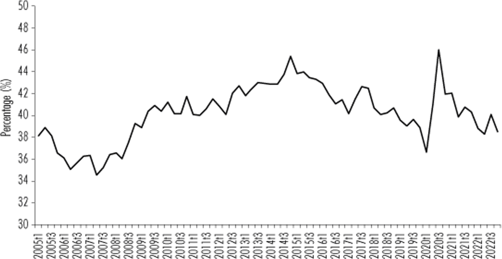
Source: compiled by the authors with information from CONEVAL (2023).
Figure 1 Evolution of the percentage of the population living in labor poverty, 2005q1-2022q4
The labor poverty rate seems to respond mainly to the income component. Esquivel (2023) points out that the increase between 2006 and 2015 is due to a stagnation in the population's income. Meanwhile, the downward phase before the pandemic can be explained by the fact that labor poverty is almost non-existent in the formally employed population, a phenomenon of informality that reduces all labor poverty.
Figure 2 shows the income mentioned above. First, it highlights the fact that both labor income deflated by the National Consumer Price Index (NCPI) and labor income deflated by the value of the basic food basket (FB) report a different trajectory from GDP per capita until 2014q4 when all three incomes enter an upward phase. This is because labor income measures only a part of the GDP per capita, as seen from the income side. In this respect, it is worth noting that labor income increased slightly until shortly before the financial crisis and, after that, it entered a downward phase until 2014q4. Meanwhile, following that crisis, GDP per capita entered an upward phase until the Covid-19 crisis, the breaking point of the three series. Finally, in the last eight quarters available, the three series entered an upward phase.
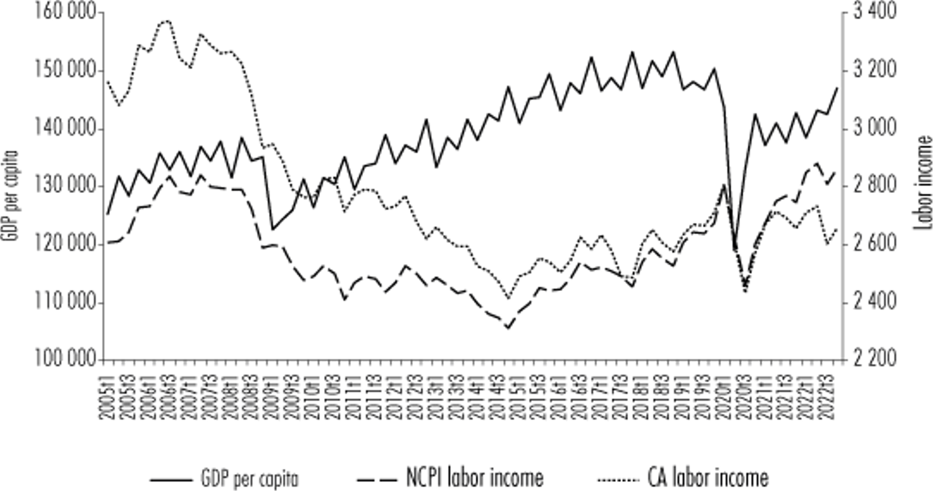
Source: compiled by the authors with data from INEGI (2023b) and CONEVAL (2023).
Figure 2 Evolution of real per capita output and real labor income, 2005q1-2022q4
Figure 3 shows the evolution of general inflation and the growth rate of poverty lines, in other words, inflation of poverty and extreme income poverty. The most noteworthy fact is that poverty line inflation is more volatile than general inflation in most of the samples; however, from 2020 onwards, it seems to behave in the same way. Nevertheless, the poverty lines represent the basic needs and basic food needs that the population would need to access, which could, in turn, imply a greater relationship between these phenomena and labor poverty.
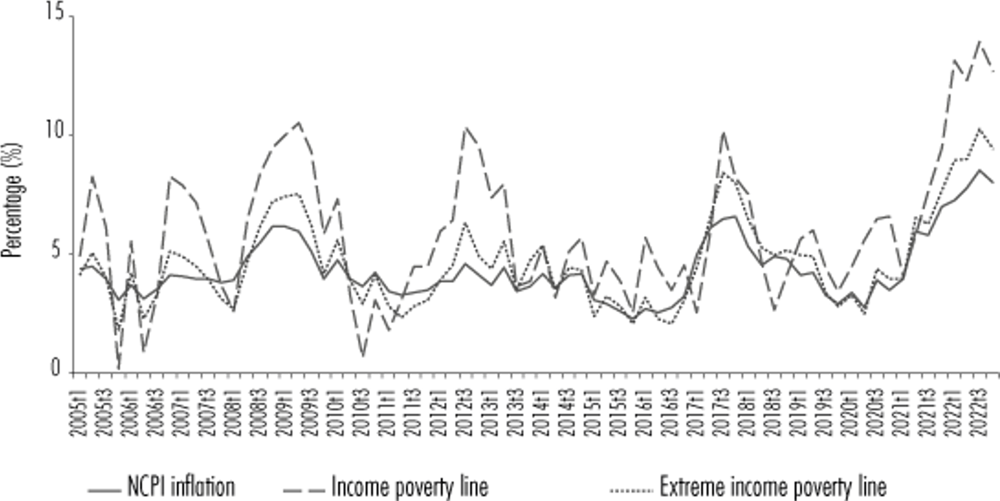
Source: compiled by the authors with data from INEGI (2023b) and CONEVAL (2023)
Figure 3 Inflation and growth rates of poverty and extreme income poverty lines, 2005q1-2022q4
These facts reveal several relevant implications. First, labor income represents 60% of household income (INEGI, 2021). Second, labor income is the reference for measuring labor poverty (CONEVAL, 2023). Third, the monetary policy transmission channels of the Bank of Mexico (Banxico, n.d.) indicate that the interest rate impacts future spending by discouraging investment and consumption, decreasing aggregate demand and, therefore, inflation. Finally, other prices impact the welfare of families, such as the value of basic food baskets.
In this respect, replacing GDP per capita with labor income and general inflation by the inflation of the two poverty lines would show that monetary policy not only has effects on aggregate variables but also has an impact on households and their members and therefore, on poverty, demonstrating the need to rethink not only the current transmission channels and the effects of each policy decision on the interest rate, but also to rethink the objectives of the banks.
Regarding the econometric methodology, a VAR model in differences3 is estimated for each scenario. The order of integration is analyzed using the Augmented Dickey-Fuller (ADF) test. Furthermore, to analyze whether there is a short and long-term macroeconomic relationship with poverty, a cointegration model with error correction is estimated, following the procedure of Engle and Granger (1987).
In this respect, the VAR model can be described as follows:
where Yt is the vector of the model's endogenous variables, Yt-1 is the vector of the k-period lagged Variables, A is the parameter matrix, and Ut is the vector of the error term.
To select the optimal number of lags in the VAR models, we followed the recommendations of Catalán (n.d.) and Loría (2007), which used the information criteria and the final forecast error as decision criteria. Furthermore, based on Lütkepohl (2005), the test of the stability assumption that takes into consideration the eigenvalues of the A matrix and the correct specification tests were used, especially the autocorrelation tests: if a VAR with ρ lags does not present autocorrelation, it should be chosen for the impulse response analysis. In this respect, the impulse response analysis is performed using the Cholesky breakdown.
Where Pobt is labor poverty, Xt is the vector of explanatory variables of the scenarios (income, inflation and interest rate), γ is the estimator associated with the error correction model (ECM). In other words, the lagged error series of the long-term equation, and vt is the error related to this specification.
The equilibrium relationship is tested by estimating the long-term relationship with the ADF test. Finally, its correct specification is checked using conventional tests.
4. Econometric estimates of the scenarios of interest
Next, we seek to test whether there is a mechanism that associates macroeconomic fundamentals with the poverty rate. In this respect, the scenarios contribute to a better understanding of shocks to the product, the effects on inflation, the monetary policy response of central banks and the change in labor poverty.
The series were transformed into natural logarithms. Table 1 shows the summary statistics and the z-statistic of the ADF unit root test for the seven variables in relation to level and first difference. The ADF test was performed without intercept or trend, with four lags. In addition, to confirm these results, the Z(t) statistic of the Phillips-Perron (PP) test, including trend and constant with the same lags, is reported. The series is order 1 stationary.
Table 1 Summary statistics and unit root tests on level and first differences
| GDPpc | Lab_inc | Inf | IPL | EIPL | r | PL | ||||||||
| x | Δ(x) | x | Δ(x) | x | Δ(x) | x | Δ(x) | x | Δ(x) | x | Δ(x) | x | Δ(x) | |
| µ | 11.8 | 0.00 | 7.92 | 0.00 | 0.39 | 0.03 | 0.01 | 0.00 | 0.01 | 0.00 | 1.77 | 0.00 | 3.69 | 0.00 |
| σ² | 0.06 | 0.04 | 0.09 | 0.03 | 0.86 | 1.01 | 0.01 | 0.02 | 0.01 | 0.02 | 0.33 | 0.09 | 0.06 | 0.03 |
| ADF | 0.56 | -4.27 | -1.12 | -3.76 | -1.78 | -3.15 | -0.02 | -4.99 | -0.55 | -5.96 | 0.18 | -2.62 | 0.26 | -4.07 |
| PP | -3.48 | -15.7 | -1.54 | -7.88 | -6.18 | -11.2 | -7.98 | -14.6 | -8.02 | -17.8 | -1.80 | -3.43 | -2.11 | -9.31 |
Notes: x: series on tevel; Δ(x): series on first difference. μ: mear; σ2 standard deviation. GDPpc: GDP per capita; Lob_inc: real labor income; Inf: inflation rote; IPL Inflation o( the income poverty line; EIPL: inflation of the extreme income poverty line; r:90day THE; Lft Trbor poverty.
Source: own estimates.
Scenario I. GDP per capita, inflation, interest rate and labor poverty
The first model corresponds to an estimation that links the main macroeconomic variables with labor poverty. Table 2 shows the information criteria associated with different specifications of the VAR model. It was decided to estimate specifications from 1 to 8 lags, or lagged effects from one quarter to two years. The Jarque-Bera normality and LM autocorrelation tests with 4 lags are also shown as criteria for choosing the best estimation.
Table 2 Information criteria and teste of correct specification on ρ order VARs: Scenario I
| ρ-lags | FFE | AIC | HQIC | SBIC | JB | LM |
| 0 | 3.00E-09 | -19.916 | -19.916 | -19.916 | - | - |
| 1 | 7.70E-10 | -21.294 | -21.066 | -20.700 | 0.000 | 0.000 |
| 2 | 4.10E-10 | -21.945 | -21.4875* | -20.7553* | 0.000 | 0.237 |
| 3 | 4.10E-10 | -21.963 | -21.277 | -20.179 | 0.001 | 0.776 |
| 4 | 4.00E-10 | -22.041 | -21.126 | -19.662 | 0.106 | 0.401 |
| 5 | 3.5e-10* | -22.274 | -21.131 | -19.300 | 0.801 | 0.413 |
| 6 | 4.50E-10 | -22.203 | -20.831 | -18.634 | 0.387 | 0.284 |
| 7 | 6.60E-10 | -22.045 | -20.444 | -17.881 | 0.000 | 0.167 |
| 8 | 5.40E-10 | -22.598* | -20.768 | -17.840 | 0.141 | 0.045 |
Notes. FFE: Final forecost error; AIC: Akaike criterion; HQIC: Honnon^uin criteria; SBIC: Bayesian criterion. For mote details on tftese criteria, see Lütkepohl (2005). Resuhs witfi * indicate the best model according to the estimated criterion parameters. JB: Jaique Bera nonnality test. LM: Autocorrelation test on Lagrange multipters. The associated pvalues are reported. For the LM, the probabi1ty associated with the fourth Iag is reported. All specifications incorporate the following dummies: 2009ql, 2020q2 and 2020q3.
Source: own estimates.
The results in Table 2 are varied. However, using the correct specification tests, the model whose lags provide more information for understanding the phenomenon is the order 5 VAR. The analysis strategy is as follows: Figure 1 shows the impulse analysis of the macroeconomic variables—income, inflation and interest rate—in labor poverty, while Figure 2 reports the impulse and causality response of the three equations (Carlin and Soskice, 2015).
The results in Figure 4 regarding the response of the labor poverty rate to a shock in the system variables show: a) a boost in income corresponds to a correction in long-term poverty by equilibrating it to four periods after a shock; b) the effect of inflation lingers on poverty by moving as a wave. In this respect, it diverts it from its equilibrium path; c) the effect of a boost in the interest rate increases poverty in the first period. However, the effect dissipates quickly over time and d) poverty per se does not seem to have inertial effects on itself.
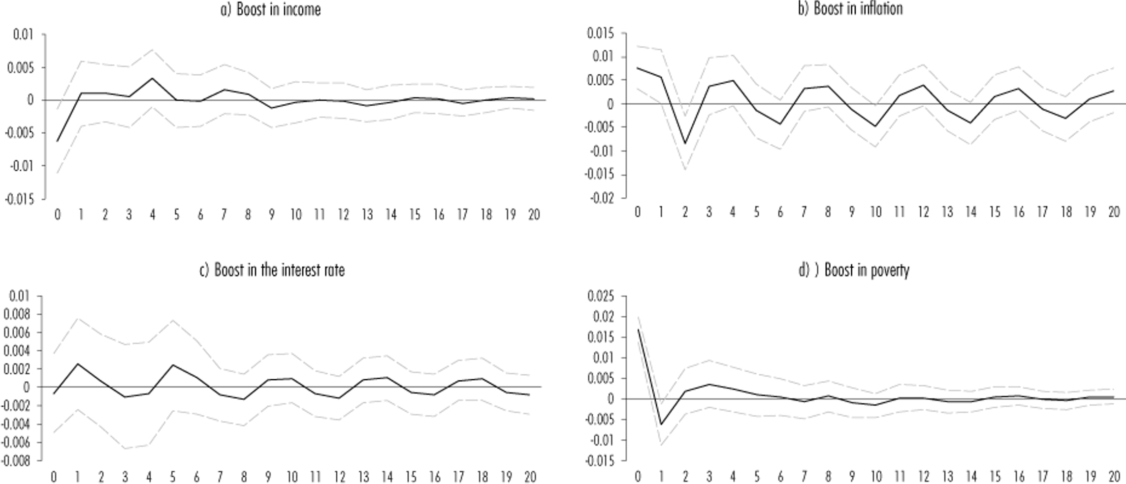
The effects of Figure 5 indicate that a) an income shock diverts inflation from its equilibrium for several periods; b) the Central Bank raises the interest rate to control the shock with some lag periods before returning the economy to its equilibrium; c) this increase in the interest rate causes delays in the adjustment of inflation; finally, d) this increase diverts the product from its long-term trend, as it takes some periods to return to equilibrium.
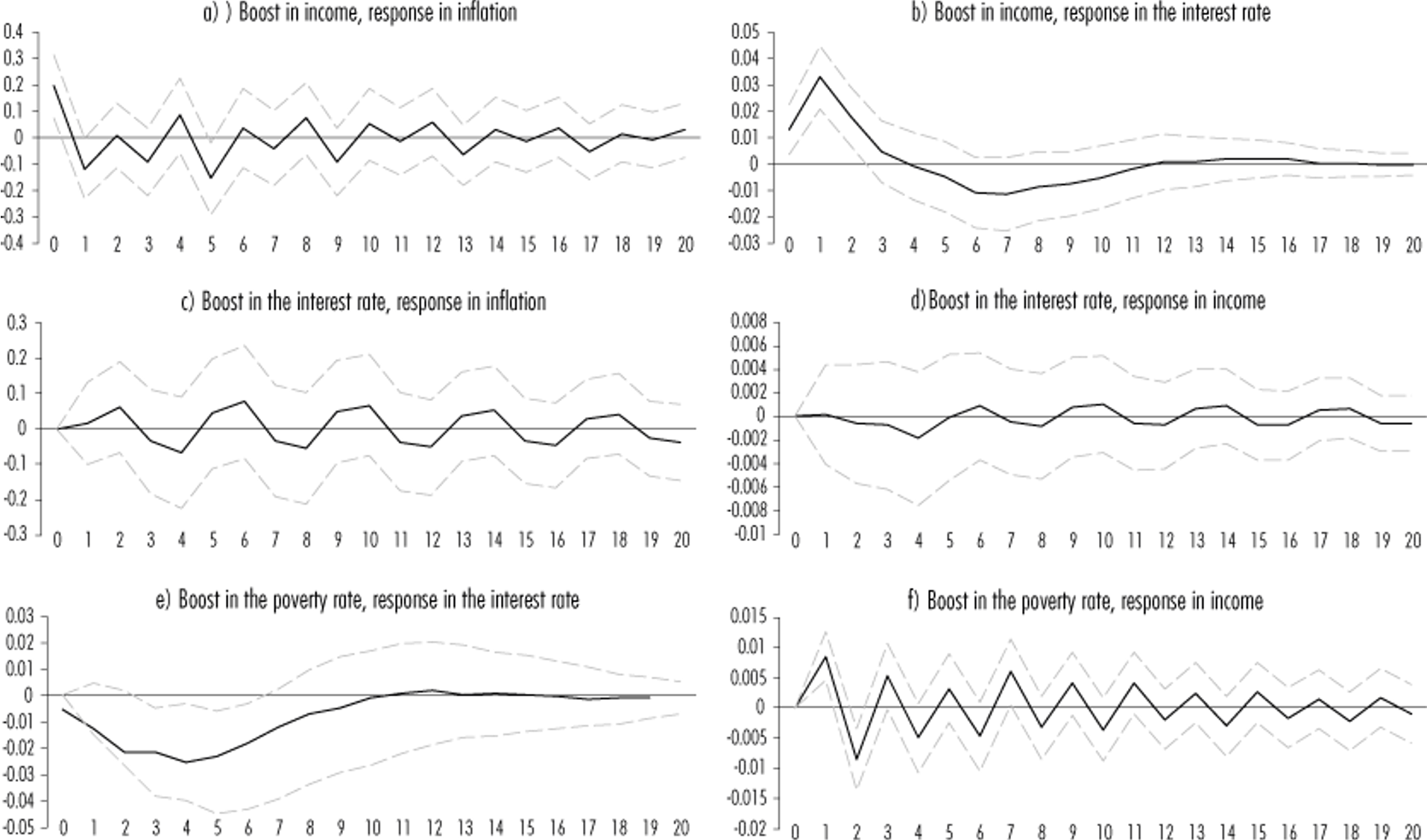
In turn, two more effects are added: the increase in poverty and its impact on interest (e) and income (f). An increase in poverty results in a reduction in the interest rate that lasts about five periods before it begins to return to its normal level while diverting income from its equilibrium for several periods.
The mechanism by which the effect in (e) occurs could be due to the causes that generated the increase in poverty. Since this population is mainly salaried (Department of Economic and Social Affairs, 2009), this may be due to the rise in unemployment, which causes lower wages. In this respect, based on the analytical framework of Carlin and Soskice (2015), there is less inflation than there should be, which could deviate it from its target. This would lead to an adjustment by lowering the interest rate, implying an increase in income, leading to a recovery in wages and, subsequently, inflation, returning the system to its long-term equilibrium.
Scenario II. Real labor income, income poverty line, interest rate and labor poverty
Table 3 reports the selection of lags of the VAR model of this scenario and the correct specification tests for models with up to 8 lags. In this case, it was decided to estimate an order 5 VAR. Although no information criterion selects it, it complies with the assumptions on the error and the stability of the system (Lütkepohl, 2005).
Table 3 Information criteria and correct specification tests on the p order VARs: Scenario Il
| ρ-lags | FPE | AIC | HQIC | SBIC | JB | LM |
| 0 | 1.80E-13 | -18.007 | -17.845 | -17.595 | ||
| 1 | 7.60E-14 | -18.866 | -18.489 | -17.906 | 0.000 | 0.000 |
| 2 | 3.80E-14 | -19.553 | -18.960 | -18.0433* | 0.159 | 0.001 |
| 3 | 2.3e-14* | -20.094 | -19.2857* | -18.035 | 0.024 | 0.111 |
| 4 | 2.60E-14 | -19.995 | -18.971 | -17.388 | 0.002 | 0.063 |
| 5 | 3E-14 | -19.929 | -18.690 | -16.773 | 0.069 | 0.219 |
| 6 | 3.10E-14 | -19.993 | -18.538 | -16.287 | 0.081 | 0.464 |
| 7 | 4.10E-14 | -19.879 | -18.209 | -15.625 | 0.037 | 0.178 |
| 8 | 2.70E-14 | -20.5013* | -18.615 | -15.698 | 0.000 | 0.200 |
Notes: FPE: Final forecast error; AlC: Akaike criterion; HOK: HannarrOuin criteria; SBIC: Bayesian criterion. For more details on these criteria, see Lütkepohl (2005). Results with * indicate the best model according to the estimated criterion porameters. JB: Jarque Bera normality test. LM: Autocorrelation test on Lagrange multipliers. The associated pvolues are reported. For the LM, the probability associated with the Iourth krg is reported. All specifications incorporate the (allowing dummies: 2020q2, 2020q3 and 2020q4.
Source: own estimates.
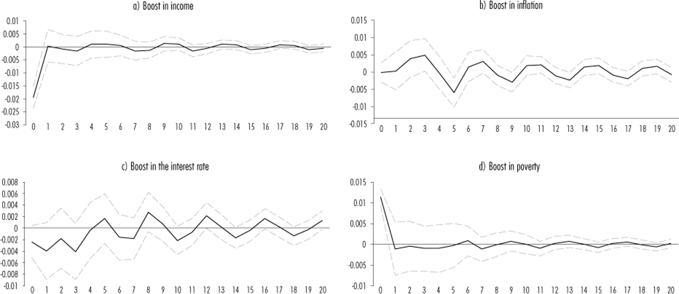
The results with real labor income and income poverty line inflation do not seem to alter the impulse responses of scenario I in relation to the labor poverty rate (see Figure 4). A boost in a) income drives poverty to equilibrium in the two periods following the shock; b) IPL inflation has long-term effects on poverty, taking longer to return to its initial value; c) the same happens with the interest rate; d) while poverty by itself does not seem to have inertial effects.
Scenario III. Labor income, extreme income poverty line, interest rate and labor poverty
Unlike the previous scenario, scenario III substitutes inflation of the IPL for that of the extreme income poverty line. In this respect, given the information criteria and the specification tests, the lags that provide more information to the model are order 2. The results for this and the models up to 8 lags are reported in Table 4.
Table 4 Information criteria and tests of correct specification on the VARs of order ρ: Scenario Ill
| ρ-lags | FPE | AIC | HQIC | SBIC | JB | LM |
| 0 | 2.30E-13 | -17.730 | -17.568 | -17.318 | - | - |
| 1 | 7.90E-14 | -18.825 | -18.4481* | -17.8646* | 0.000 | 0.095 |
| 2 | 6.6e-14* | -19.020 | -18.428 | -17.511 | 0.051 | 0.095 |
| 3 | 7.10E-14 | -18.963 | -18.155 | -16.905 | 0.036 | 0.082 |
| 4 | 8.30E-14 | -18.853 | -17.829 | -16.246 | 0.004 | 0.018 |
| 5 | 1.1E-13 | -18.601 | -17.362 | -15.445 | 0.060 | 0.038 |
| 6 | 1.00E-13 | -18.784 | -17.329 | -15.079 | 0.040 | 0.075 |
| 7 | 1.10E-13 | -18.840 | -17.170 | -14.586 | 0.001 | 0.005 |
| 8 | 9.50E-14 | -19.2293* | -17.343 | -14.426 | 0.000 | 0.094 |
Notes: FPt Final forecast error; AlC: Akaike criterion; HQIC: HonnandJuin criterio; SBIC: Bayesian criterion. For more details on these criteria, see Ludcepohl (2005). Results with * indicate the bestmodel according to the estimated criterion porameters. JB: Jarque Bera normality test. LM: Autocorrekrtion test on Lagronge multipliers. The associated puolues are reported. For the LAE, the probability associated with the fourth Iag is reported. All specifications incorporate the following dummies: 2020q2,2020q3 and 2020q4.
Source: own estimates.
The results in Figure 7 indicate that a) income quickly balances poverty after a shock; b) inflation of the basic food basket first decreases and then increases the poverty rate. However, the adjustment takes place relatively quickly; c) the interest rate, like income, quickly adjusts income, bringing poverty toward its equilibrium value, while d) poverty does not generate inertia on its own.
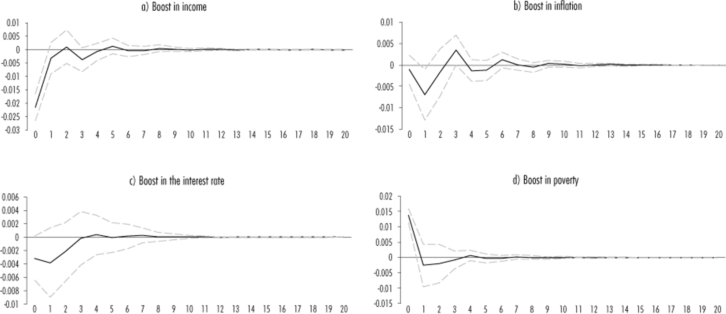
The effect in b) could be counterintuitive because an increase in the value of the basic food basket would have to increase poverty, at least in the early periods after the shock. However, with unequal income distribution, an increase in the poverty line does not necessarily translate into an increase in poverty (Shahrier and Lian, 2018). An increase in the inflation of the basic food basket, by reducing purchasing power, incentivizes employment as work is less costly due to inflation, increasing income and, therefore, reducing poverty (Department of Economic and Social Affairs, 2009). One of our objectives is to study the links between the short- and long-term discussed below.
Cointegration analysis of the different scenarios
This section estimates the cointegration equation for the different scenarios. This is necessary to study the link between the short-term estimation of the main variables of interest and the long-term path of the labor poverty rate. In this respect, Engle and Granger’s representation theorem (1987) suggests using an error correction model (ECM) to estimate such a purpose.
Table 5 reports the unit root test ADF on these scenarios’ long-term equation error series. The reported results indicate that a cointegration relationship exists for each of the scenarios considered.
Table 5 Unit root test on Hie bng-term equation error series
| Scenario | Unit root test |
| Scenario I | -2.95 |
| Scenario II | -2.82 |
| Scenario III | -2.87 |
Source: own estimates. ADF test without intercept, trend and with four logs.
Table 6 reports the long-term estimation and the cointegration estimation for each of the scenarios. It is striking that income is not significant in the long-term relationship for scenario I. Furthermore, the opposite of the expected sign is reported, and labor income does have an impact on poverty (II and III). This result does not necessarily imply that income does not reduce poverty (I) but rather that general income does not have a direct impact on labor poverty since it does so through its labor component.
Table 6 Estimation of the error correctioon model for labor poverty
| Long term | Short term | |||||
| (1) | (2) | (3) | (4) | (5) | (6) | |
| Scenario | I | II a,b | III a,c | I | II a,b | III a,c |
| Income | 0.0600 | -0.498*** | -0.503*** | |||
| (0.0998) | (0.0353) | (0.0352) | ||||
| Inflation | 0.0916*** | 0.267 | 0.147 | |||
| (0.0270) | (0.221) | (0.189) | ||||
| Interest rate | -0.133*** | -0.0660*** | -0.0648*** | |||
| (0.0141) | (0.00994) | (0.00994) | ||||
| ΔL3.Labor povertyl | 0.00198 | -0.0113 | 0.00812 | |||
| (0.0919) | (0.0502) | (0.0504) | ||||
| ΔIncome | -0.351*** | -1.007*** | -1.015*** | |||
| (0.0869) | (0.0651) | (0.0668) | ||||
| ΔL1.Income | -0.521*** | |||||
| (0.0860) | ||||||
| ΔInflación | 0.997** | -0.281*** | -0.147 | |||
| (0.427) | (0.103) | (0.0893) | ||||
| ΔL1.Inflación | -2.174*** | |||||
| (0.422) | ||||||
| ΔInterest rate | -0.0734*** | -0.0800*** | ||||
| (0.0209) | (0.0209) | |||||
| ΔL4.Interest rate | 0.0185 | |||||
| (0.0406) | ||||||
| L.ECM | -0.178* | -0.419*** | -0.489*** | |||
| (0.0907) | (0.0950) | (0.0925) | ||||
| Constant | 2.812** | 7.752*** | 7.787*** | 0.0145** | -0.00265 | -0.00275* |
| (1.114) | (0.270) | (0.269) | (0.00673) | (0.00161) | (0.00162) | |
| Observations | 72 | 71 | 71 | 67 | 68 | 68 |
| R² | 0.655 | 0.890 | 0.889 | 0.545 | 0.864 | 0.860 |
| R²-adj | 0.640 | 0.886 | 0.884 | 0.491 | 0.853 | 0.849 |
| Jarque-Bera | 0.828 | 0.009 | 0.131 | 0.755 | 0.884 | 0.581 |
| LM | 0.246 | 0.016 | 0.013 | 0.725 | 0.280 | 0.160 |
| Breusch-Godfrey | 0.000 | 0.004 | 0.005 | 0.967 | 0.505 | 0.660 |
| Ramsey-reset | 0.000 | 0.054 | 0.005 | 0.159 | 0.611 | 0.508 |
Notes: Standard error in parentheses. The probability ossociated with the test statistics is reported. The LM and Breusch-Godfrey testwos constructed with lags, a Refers to real labor income; b refers to IPLinflation; c refers to EIPL inflation. *** p<0.01; ** p<0.05; * p<0.1.
Source: own estimations.
Regarding the effects of inflation in scenario I, the expected sign is reported and is statistically significant; in other words, an increase in inflation increases poverty. However, this does not occur in scenarios II and III. The long-term relationships with the interest rate are all significant and negative, so an increase in interest reduces poverty. This indicates that a policy that prioritizes a restrictive monetary policy, favoring low inflation, corresponds to lower poverty.
The correct specification tests give rise to cointegration by error correction. In this respect, the ECM reports the expected sign, which is significant, so that, in each period, the deviation from equilibrium of the short-term effects is corrected. The transmission mechanism is faster for scenarios II and III than in I.
In this respect, an increase in income reduces the poverty rate in all three scenarios. However, labor income reduces poverty more than proportionally in the short run. For example, in scenario III, a 1% increase in income decreases labor poverty by 1.015%. In the case of scenario I, this relationship also occurs in the first income lag.
The effect of inflation in I in the first lag is negative; in other words, an increase in inflation reduces poverty. However, without lag, it is positive, and the effect described in scenario III of the impulse-response analysis is, therefore, very short-term: inflation is detrimental to poverty.
The interest rate has no short-term effect on poverty in scenario I, but it does in scenarios II and III. In other words, a quick response of monetary policy is crucial to keeping inflation low and stable and reducing poverty. Finally, poverty by itself does not have an inertial effect, a result that was also shown in the impulse-response analysis.
Returning to the positive result of the first inflation lag in scenario I on the interest rate, this effect could clarify the relationship between monetary policy and poverty. In the context of the Carlin and Soskice (2015) model, an episode that impacts inflation involves a revision of workers' wages and an adjustment to prices.
Depending on the power, both in price and wage setting, this increase in inflation—decrease in poverty—suggests two possibilities: the first is that workers could negotiate higher wages, thus increasing income and, therefore, reducing poverty. However, as mentioned, a slight increase would be enough to reduce labor poverty in unequal societies effectively. The second is that workers would be willing to be employed for lower wages so that labor poverty could be reduced due to increased income earners per household.
However, the contemporaneous effect is that the increase in inflation is detrimental to poverty. The distributional process explained above could be solved with increased timeliness if monetary policy provides a favorable response through the interest rate, as the results of the models suggest. In this respect, a low and stable inflation environment benefits the lower-income population.
5. Conclusions
The main result suggests that a monetary policy that promotes low inflation will reduce the labor poverty rate in Mexico. In this respect, the reaches of monetary policy are broader than acknowledged in the literature and inside central banks.
Throughout the analyzed period, the Mexican economy was characterized by cyclical behavior in most economic variables reviewed in this research. However, to contextualize the econometric results obtained, we should not lose sight of the two significant contractions in the GDP in 2009 and 2020 and inflationary episodes throughout the years considered.
Additionally, in the last five years (2018-2023), the Mexican economy reported an increase in minimum wages, a factor not recorded in several previous decades. After a five-year period of minimum wage increases well above inflation, although such a trend should continue in the short term, a suitable correction to the interest rate is also required in the context of a marked downward trend in the inflation rate and the monetary value of the basic food basket, in both cases, falling by 2025.
The results presented here assume that labor poverty is a given. In this respect, we need a better understanding of the main factors determining whether a person is subject to labor poverty. A better understanding of such factors will allow us to obtain more robust conclusions about the relationship between poverty and macroeconomics, economic policy, social policy, fiscal policy, etc. However, that is beyond the scope of this research.
Finally, the relationship between macroeconomics and poverty should be explored in greater detail from a theoretical and empirical perspective. The results presented here are hoped to stimulate discussion about the need to promote policies that correct and reduce poverty for the benefit of society as a whole.
REFERENCES
Abdulrahman, I. A., Akanbi, S. B. y Oniyide, G. D. (2023). Impact of monetary policy on poverty reduction in Nigeria. African Journal of Economic Review, 11(1).https://www.ajol.info/index.php/ajer/article/view/240131 [ Links ]
Ames, B., Brown, W., Devajaran, S. y Izquierdo, A. (2001). Macroeconomic policy and poverty reduction. International Monetary Fund | The World Bank. https://www.imf.org/external/pubs/ft/exrp/macropol/eng/#2 [ Links ]
Azis, I. (2008). Macroeconomic policy and poverty. Tokio: ADBI Discussion Paper 111. https://www.adb.org/publications/macroeconomic-policy-and-poverty [ Links ]
Banco de México (Banxico) (s.f.). Efectos de la política monetaria sobre la economía. México: Banco de México. https://www.banxico.org.mx/politica-monetaria/d/%7BCE7DEA10-0015-1138-4A2F-F3580416D34F%7D.pdf [ Links ]
______ (2024). Sistema de Información Económica. https://www.banxico.org.mx/SieInternet/ [ Links ]
Campos, R. y Monroy, L. (2016). La relación entre crecimiento económico y pobreza en México. Investigación Económica, 75(298 ). https://doi.org/10.1016/j.inveco.2016.11.003 [ Links ]
Carlin, W. y Soskice, D. (2015). Macroeconomics. Institutions, instability, and the financial System. Oxford University Press. [ Links ]
Cashin, P., Mauro, P., Patillo, C. y Sahay, R. (2001). Macroeconomic policies and poverty reduction: Stylized facts and an overview of research. IMF Working Paper Research Department. https://www.imf.org/en/Publications/WP/Issues/2016/12/30/Macroeconomic-Policies-and-Poverty-Reduction-Stylized-Facts-and-an-Overview-of-Research-15334 [ Links ]
Catalán, H. (s.f.). Econometría y análisis de políticas sociales. CEPAL. https://www.cepal.org/sites/default/files/courses/files/hc_3_especificacion_var.pdf [ Links ]
Consejo Nacional de Evaluación de la Política de Desarrollo Social (CONEVAL) (2023). Medición de la pobreza. https://www.coneval.org.mx/Medicion/Paginas/PobrezaInicio.aspx [ Links ]
Department of Economic and Social Affairs (2009). Rethinking poverty. Report on the world social situation 2010. United Nations. [ Links ]
Engle, R. y Granger, C. (1987). Co-Integration and error correction: Representation, estimation, and testing. Econometrica, 55(2). https://doi.org/10.2307/1913236 [ Links ]
Esquivel, G. (2023). La pobreza laboral en México, a la baja. Economía UNAM, 20(59). https://doi.org/10.22201/fe.24488143e.2023.59.795 [ Links ]
Ekobena, S. (2014). Does monetary policy really affect poverty?https://www.cepweb.org/wp-content/uploads/2014/04/CEP_Atlanta_Fed_Fouda.pdf [ Links ]
Instituto Nacional de Estadística y Geografía (INEGI) (2021). Encuesta Nacional de Ingresos y Gastos de los Hogares (ENIGH). 2020 Nueva serie. https://www.inegi.org.mx/programas/enigh/nc/2020/ [ Links ]
______ (2023a). Encuesta Nacional de Ocupación y Empleo (ENOE), población de 15 años y más de edad. https://www.inegi.org.mx/programas/enoe/15ymas/ [ Links ]
______ (2023b). Banco de Información Económica. https://www.inegi.org.mx/app/indicadores/?tm=0#bodydataExplorer [ Links ]
Loría, E. (2007). Econometría con aplicaciones. Pearson Educación. [ Links ]
Lütkepohl, H. (2005). New introduction to multiple time series analysis. Springer. [ Links ]
Mendoza Cota, J. y Torres Preciado, V. (2022). Remittances and poverty: new macroeconomic evidence at the state level in Mexico. Revista de Economía Regional y Sectorial, 14(2).https://www.redalyc.org/articulo.oa?id=431571245013 [ Links ]
Romer, C. y Romer, D. (1998). Monetary policy and the well-being of the poor. NBER Working Paper 6793. doi:10.3386/w6793 [ Links ]
Saeed, M. (2020). The effects of monetary policy on poverty alleviation in Pakistan. Journal of Research & Reviews in Social Sciences Pakistan, 3(1). http://dx.doi.org/10.2139/ssrn.3693375 [ Links ]
Setterfield, M. (2006). Is inflation targeting compatible with post Keynesian economics? Journal of Post Keynesian Economics, 28(4). http://www.jstor.org/stable/4538996 [ Links ]
Shahrier, N. y Lian, C. (2018). The impact of monetary and fiscal policies on poverty incidence using financial computable general equilibrium (FCGE): Case evidence of Thailand. https://www.bsp.gov.ph/About%20the%20Bank/Events/IRC/papers/2018_BSP-IRC_07_paper.pdf [ Links ]
Sims, C. (1980). Macroeconomics and Reality. Econometrica , 48(1). https://doi.org/10.2307/1912017 [ Links ]
Torres, F. y Rojas, A. (2015). Política económica y política social en México: desequilibrio y saldos. Problemas del Desarrollo. Revista Latinoamericana de Economía, 46(182). https://doi.org/10.1016/j.rpd.2015.06.001 [ Links ]
1This paper does not necessarily reflect the opinion of CONEVAL. Responsibility for the information, errors and omissions is the responsibility of the authors.
2Labor poverty is estimated based on the National Survey of Occupation and Employment and its new version (ENOE and ENOE-N) carried out by the National Institute of Statistics and Geography (INEGI, 2023a). In this respect, it is important to note that this source reports a shortfall in the second quarter of 2020 due to the fact that it was interrupted by the onset of the Covid-19 pandemic. To account for this missing value, we opted for a simple intrapolation between the values for the first and third quarters of 2020.
3This responds to a research need rather than to the methodology of the VAR models themselves. For example, Sims (1980) argues in favor of estimation in levels because stationary series lose information on the variables of interest.
Received: August 30, 2023; Accepted: January 30, 2024
 Este es un artículo publicado en acceso abierto bajo una licencia Creative Commons
