INTRODUCTION

Signal analysis is essential in many engineering fields, including power systems, vibration analysis, voice recognition, radar applications, biomedical engineering, and digital communications. Because it allows obtaining relevant features regarding system information. The human body has different systems, such as the cardiovascular, nervous, and respiratory system, among others^[1]. From these systems, signals can be obtained that provide relevant information. These signals are processed for analysis^[2][3], which leads to their quantization, causing quantization error. These signals can not only be affected by quantization error but also by other errors caused by measurement instrument components or incorrect usage. One solution to this issue is the implementation of a methodology that considers noise filtering and achieves instantaneous estimates without the need for a sample window for estimation.

The measurement of biomedical signals is a cornerstone of modern healthcare, providing critical insights into physiological processes and aiding in the diagnosis and treatment of various medical conditions. Common examples of biomedical signals are electrocardiograms (ECG), electroencephalograms (EEG), and blood pressure measurements. These signals are crucial for monitoring patient health, conducting medical research, and developing new medical technologies. The precision and capabilities of biomedical signal measurement depend on sensors and signal processing techniques. Digital Signal Processing (DSP) techniques enable the extraction of meaningful information from noisy signals, improving diagnostic accuracy^[4]. Therefore, the rates of change in biomedical signals are part of their analysis.

Below are some methodologies that can be implemented in signal estimation, which can also estimate the rate of change in the signal. The Savitzky-Golay (Sgolay) method includes the use of data windows^[5][6], introducing a delay in its estimates. In^[7][8], the discrete wavelet transform is implemented to cancel disturbances in ECG caused by devices or movements. However, even when the sample window size can be narrow depending on the signal resolution to be estimated, a sample window is still necessary for information estimation. On the other hand, the Nonlinear Tracking Differentiator (NTD) method^[9][10] requires an adjustment parameter, which consequently implies a drawback since this parameter needs to be calibrated with respect to the signal to be estimated, leading to potentially suboptimal or highly suboptimal estimates. In response to these limitations and based on the results obtained from the methodology used in^[11][12] for phasor estimation, it was proposed to employ a methodology that enables instant estimations. This methodology is grounded in the implementation of a signal model that includes its respective derivatives, all within a state transition matrix. With a zeroth-order model (approximating the signal with a zeroth-order Taylor polynomial), estimations of the electrocardiogram are obtained. By increasing the order of the Taylor polynomial, the model is modified, allowing for the estimation of signal derivatives, achieving a better response in estimation for signals corrupted by noise. This methodology surpasses the limitations of other strategies in the sense that there is no need for a sample window to perform estimations and enables a more accurate signal approximation by reducing noise. Consequently, the proposed method focuses on obtaining a more precise and comprehensive estimation in relation to the characteristics of biomedical signals. It successfully provides good estimates for signals such as electrocardiograms, cardiorespiratory signals, and blood pressure. Another method that can be implemented in the analysis of biomedical signals is the Extended State Observer (ESO), proposed for the cascade of integrator systems without measurement noise^[13][14].

In the monitoring of ECG, it is common to use modulation techniques for transmission and reception. Some techniques have been developed; for example, in^[15], a real-time algorithm for ECG-Derived Respiration is presented. In^[16], an adaptive algorithm using different modulation schemes is introduced. In^[17], a method for ECG monitoring is proposed that utilizes a transmitter-receiver system with modulation frequencies to send and receive ECG information.

Achieving a better representation of an ECG signal is another objective. For instance, in ^[18], a method to obtain a better representation of blood flow signals was proposed. In^[19], a novel ECG enhancement algorithm based on sparse derivatives is introduced. In^[20], the ECG is viewed as a quasi-periodic process and employs the unbiased finite impulse response (UFIR) smoother on optimal horizons, applied to a harmonic ECG model with good results. In^[21], a new tracking differentiator is proposed, which can synchronously filter noise and estimate the derivative of the input signal. The proposed method, based on the analysis of the rate of changes in some biomedical signals such as ECG and blood pressure, involves the development of a model using a passband signal and its derivatives. By approximating the signal and its derivatives with Taylor polynomials, it is possible to develop a state transition to implement in the Kalman filter. Since the proposed method uses Taylor polynomials, the methodology is compared with a Digital Differentiator based on Taylor Series (DDTS)^[21].

The aim of this work is to present a method to estimate the derivative signal of an ECG. With the derivative, it is possible to detect high frequencies in the ECG, which are common in coronary heart disease and useful for electrocardiographic diagnosis. In^[22], the derivative of an ECG is obtained using an electronic circuit and operational amplifier. However, in this document, the derivative is obtained mathematically, and the algorithm can be implemented in any microcontroller, DSP, FPGA, or PC. Additionally, the numerical results can be obtained in real time, and the method only needs one sample to achieve the estimate of both the signal and its derivative.

MATERIALS AND METHODS

Commonly, biological systems produce quasi-periodical signals. These signals are almost periodical signals, but with fluctuations between periods. Next, the model shown in^[12][23] for a quasiperiodic signal oscillation is presented.

We start using a periodical signal s_p (t), a fundamental approach involves to represent a periodic signal by its Fourier representation in Equation 1:

where ω₁ represents the fundamental frequency in radians per second, H is the number of harmonics considered, and c_h represents the Fourier coefficient related to the h-th harmonic.

If (1) is relaxed to allow slow variations (compared with ω₁) in c_h in both amplitude and phase, then the expression

can be used to model the fluctuation through the behavior of each coefficient, where a_h (t) and φ_h (t) now represent the amplitude and phase variation for each harmonic. Under the assumption (Equation 2), the quasi-periodic version of s_p(t) is given by

where for a real-valued signal (Equation 3), the components should meet cht_= c-h(t) for h ≠ 0, with cht_ representing the complex conjugate of c_h (t). This relaxed model offers more flexibility as it allows the description of the time-varying dynamic evolution of each harmonic. The Taylor series at t₀ can be used to represent each passband signal (Equation 4) by:

with ch(k)t0=dkchtdtkt=t0 representing the k-th derivative of the h-th harmonic at t = t₀, and εh(k+1)t (t) representing the residue due to higher-order terms.

Using (Equation 4) in (Equation 3), the following ex-pressing is obtained for the quasi-periodical signal (Equation 5):

where

represents the h-th rotated phasor, and Ε(t) represents the summation over of the residues Ε(t)=∑h=-HHεh(k+1)(t).

The relation (Equation 6) can be used to construct a transition function for the rotated phasor from time t₀ to time t. We construct it by analyzing (Equation 6) per each value of h. We separate two cases, h = 0 and h ≠ 0.

First, for h = 0, the DC component r₀ = c₀ at instant t can be related to t₀ by performing the derivation of (Equation 6) (K - 1) times (Equation 7):

where the i-th element o the vector r₀(t) ∈ ℝ^{(K + 1)} is given by the i-th derivative of the DC component c0(i)t for i = 1, … , n; and the i-th element of the j-th column of the matrix Ψ(t - t₀) ∈ ℝ^{(K + 1)×(K + 1)} is given by (Equation 8):

In a similar manner, for h ≠ 0 the k-th harmonic component h at instant t can be related to t₀ by performing the derivation of (6) (K_- 1) times, where now, due to the complex exponential function, we have (Equation 9):

In this context, the i-th element of r_h (t) ∈ ℂ^(K+1) , in (9) represents the _i -th derivative of rh(i)t and M(hω) ∈ ℂ^{(K + 1)×(K + 1)} is a lower triangular complex matrix with elements given by (Equation 10):

A discrete representation of (Equation 10) can be obtained sampling s(t) with a uniform sampling time T, and using t₀ = nT and t = (n + 1)T, it is possible to use the relations in (Equation 9) to relate the rotated phasor from sample to sample. From (Equation 9), with t₀ = nT and t = (n + 1)T we have (Equation 11):

where Φ_h(n + 1, n) = M (hθ)Ψ(T)M^-1(hθ)e^jnhθ1 works as a transition matrix from time nT to (n + 1)T, and θ₁ represents the discrete fundamental frequency in radians.

Using (Equation 11) to represent each component in (Equation 5), a model for the signal s(n) can be constructed as follows (Equation 12):

where x ∈ ℂ^{(2H + 1)(K + 1)} represents a vector formed from the union of the 2H + 1 vectors r_h, the components are ordered as follows x = [r₀r₁r_-1r₂r_-2 ...r_Hr_-H]'; thereby following (11) the matrix A ∈ ℂ^{(2H + 1)(K + 1)×(2H + 1)(K + 1)} is a block diagonal matrix given by (Equation 13):

and C ∈ ℝ ^{(2H + 1)(K + 1)} represents the synthesis of the signal from its harmonic components, according to (Equation 5) C is given by the union of (2H + 1) blocks ξ ∈ ℝ ^{K + 1} , where ξ = [1 0 ... 0].

Only for h = 0 the corresponding elements in A and x are real-valued. However, a real-valued version of (Equation 12) can be obtained using cht_= c-h(t) for h ≠ 0. We use the following linear transformation x~=Px where x~∈R(2H+1)K+1 (Equation 14):

Using the lineal transformation (Equation 14), a real-valued representation of (Equation 12) is (Equation 15):

where A~=PAP-1 and C~=CP-1 are real-valued matrices and x~=[r0 Re(r1) jIm(r1) ... Re(rh) jIm(rh)].

RESULTS AND DISCUSSION

In this section, the estimates of the TKA filter are illustrated and compared with the Sgolay, NTD, ESO, and DDTS methods. The test signals are ECG, RAW (data corresponding to heart R-wave to R-wave intervals), and blood pressure. As the first test signal, a synthetic ECG is developed with mathematical functions to obtain its derivative, using the set of derivatives of each of its functions. Hence, the estimation error in the signal and its derivative can be obtained. However, since the derivative in the measurement signals is not known, the error is only calculated with respect to the measurement signal.

Performance Results of the TKA Filter

The performance of the algorithm is showcased in this section, utilizing a polynomial approximation of K = 2 and H = 64 harmonics as detailed in Equation 4. In what follow we evaluate the capacity to reconstruct the input signal after applying the analysis and synthesis stages for the proposed realvalued TKA (Taylor-Kalman Algorithm). For the TKA, the analysis stage includes the state estimation using the Kalman algorithm, and then the synthesis stage computes a reconstruction of the input signal from the filter estimates. We also evaluate the performance of the TKA as a derivative are also computed. The proposed TKA Filter was implemented on a computer with Matlab 2016b, Intel Core i5 @ 2.6 GHz, 8.00 GB RAM, and operative system Mojave for MacOS is used.

As the PhysioNet signals^[26] have not information about the derivative of the measurement signal. There is a problem when the performance of the derivative estimation is evaluated. To solve this situation, a math model of ECG is used to create synthetic ECG signals with known derivatives, obtained with each function of (Equation 16). The used model was proposed in^[27], the synthetic ECG signal is defined as follows (Equation 16):

f0t=0, 0≤t≤200   (16.a)

f1t=a-a1001580bt-200+b22,  200≤t≤200+b (16.b)

f2t=0, 200+b≤t≤440 (16.c)

f3t=140-d100g+1c-1.1*0.3t-44020, 440≤t≤440+d7 (16.d)

f4(t)=140-d100g+1c1.1*0.6(t-[440+1.5d7])20,  440+d7≤t≤440+3d7 (16.e)

f5(t)=140-d100g+1c-1.1*0.5(t-[440+5d7])20, 440+3d7≤t≤440+6d7 (16.f)

f6t=140-d100g+1c-1.1*0.5t+44020, 440+6d7≤t≤440+d (16.g)

f7(t)=0,440+d≤t≤440+d+680 (16.h)

f8t=e-e1001580ft-680+f22, 440+d≤t≤440+d+f. (16.i)

The range for each one of the variables a ⋯ g used in the definition of the synthetic ECG is show in the Table 1.

Table 1 Parameters of the synthetic ECG signal. 

Variable	Function in synthetic ECG signal	Physiological interval
a	Amplitude of P wave	0-0.3 mV
b	Length of P wave	0-160 ms
c	Amplitude of the QRS complex	0-0.5 mV
d	Length or QRS complex	50-120 ms
e	Amplitude of T wave	0-0.8 mV
f	Length of T wave	0-300 ms
g	Amplitude of the QRS complex	0-50 mV

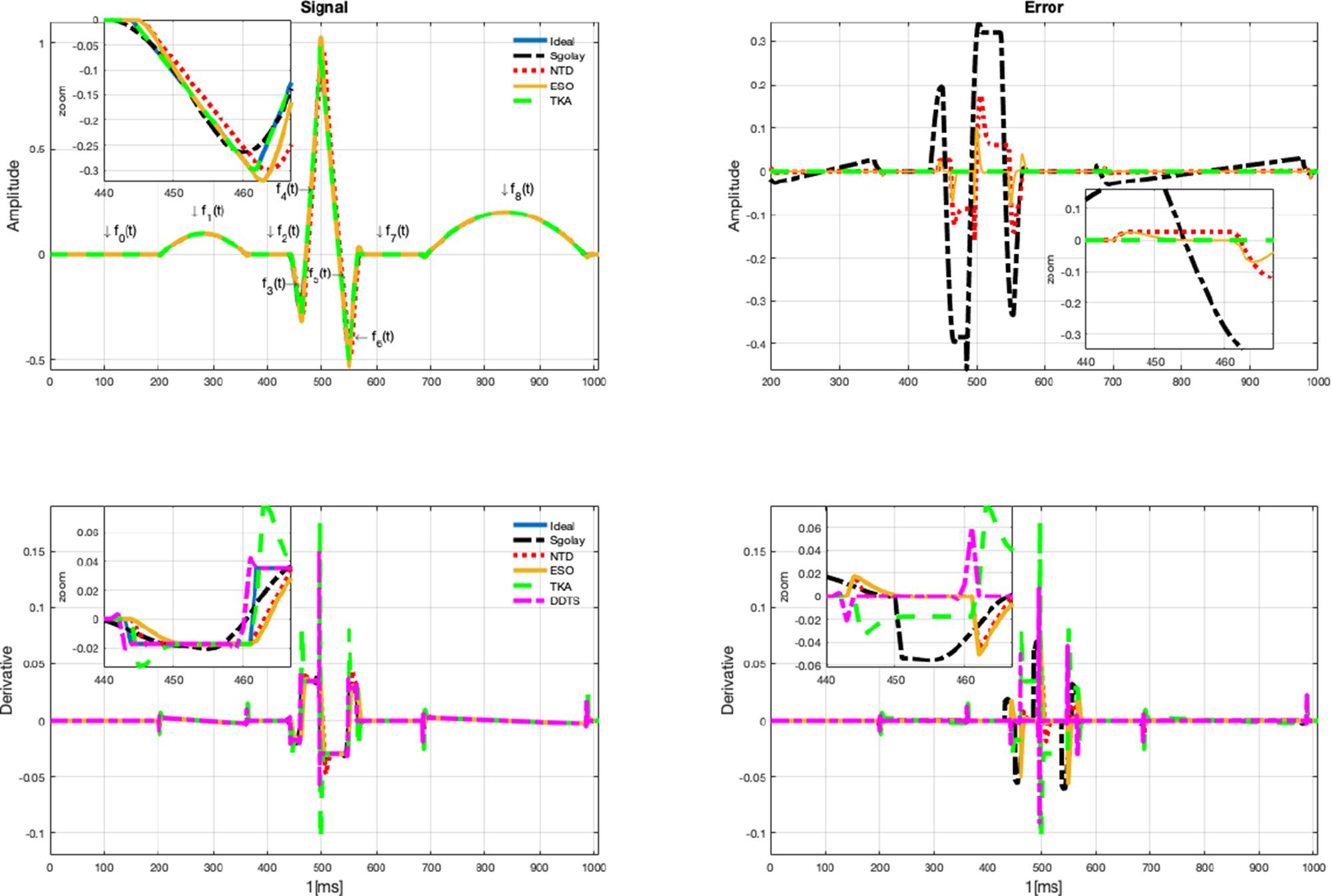
In Figure 1. The signal estimates are illustrated in top of the graph, while the derivative estimates are illustrated in bottom of the graph, the parameters used to generate the synthetic signal for this example are a = 0.1, b = 160, c = 0.096, d = 120, e = 0.2, f= 300, g = 50.

The input signal, as well as the estimates from the four algorithms, are displayed in Figure 1, (the measurement is illustrated in left top graph, and the error estimate in the right top graph). Furthermore, a zoomed-in view is offered to facilitate a closer examination of the estimation details. As it can be seen, the Sgolay estimation smooths (filters out high-frequency signals), which can lead to estimation errors in some cases or segments of the signal. On the other hand, NTD estimation provides errors in sections with abrupt changes in amplitude. And the ESO estimates have a similar behavior to the NTD but with greater amplitude. It can be observed that signal estimates provided by the proposed TKA method have the best performance. In Figure 1, left of bottom graph, the estimation of the derivative of the signal is shown, which corresponds to the same zoomed-in section of the signal. Similarly, in the derivative estimation, the Sgolay method tends to smooth the signal, NTD method provides a significant number of errors when the signal exhibits rapid changes in amplitude. It is important to remark that no additional differentiator algorithms are needed to compute the estimation of the derivative when the proposed Kalman algorithm is used. Also, the error in derivative estimation is shown in the bottom right graph in Figure 1. When an abrupt change in the signal occurs, the estimations have considerable errors, with better estimates obtained using the ESO and DDTS methods. However, the measurement signals are smoother than the synthetic signal.

Figure 1 Synthetic ECG signal and derivative estimates with Sgolay, NTD, ESO, DDTS, and TKA. 

Signal under estimation is an Electrocardiogram (ECG) signal sourced from the PhysioNet database^[26], (Signals recorded in labor, between 38 and 41 weeks of gestation; four signals acquired from maternal abdomen; direct electrocardiogram recorded simultaneously from fetal head; positioning of electrodes was constant during all recordings; Ag-AgCl electrodes (3M Red Dot 2271) and abrasive material to improve skin conductance (3M Red Dot Trace Prep 2236); bandwidth: 1Hz - 150Hz (synchronous sampling of all signals); additional digital filtering for removal of power-line interference (50Hz) and baseline drift, Sampling rate: 1 kHz; resolution: 16 bits; input ranges are included in the records in EDF format). On the other hand, the results are depicted in Figure 2, where the estimation is compared with the Sgolay, NTD, ESO and TKA, The DDTS cannot estimate the signal; it can only estimate the derivative of the signal. As can be seen in the zoomed area, better estimates of the signal are obtained with TKA. The Sgolay filter smooths the changes, while NTD and ESO provide similar estimates. However, the ESO method yields larger estimates in amplitude. The derivative estimate is shown in the graph in Figure 2. Unlike the synthetic signal, DDTS provided the worst case in the estimates and is illustrated in yellow to distinguish it from the other signal estimates. The derivative estimates with TKA improve, with regard to the synthetic signal due to the smooth changes in the amplitude of the derivative.

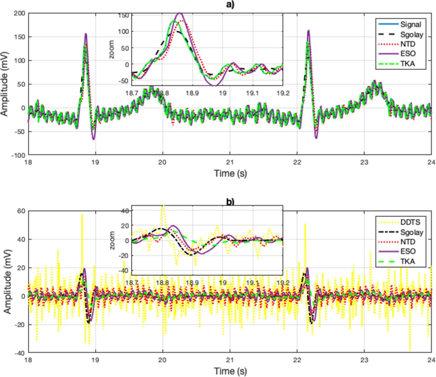
Figure 2 a) Signal reconstruction with the Sgolay, NTD, ESO and TKA methods. And Zoomed-in view of the reconstructed (estimated) signal. In b) the derivative estimates are illustrated and zoomed-in view of the derivative estimation of the signal. 

As a third example, a cardiorespiratory signal RAW (data corresponding to heart R-wave to R-wave intervals). Data correspond to heart R-wave to R-wave intervals, Oxygen consumption, and mechanical power output on a beat-tobeat basis recorded all along the graded exercise test sessions. Participants are 18 teenagers athletes (15.2±2 years) from the Regional Physical and Sports Education Centre (CREPS) of French West Indies (Guadeloupe, France)^[26]. The results obtained using the Sgolay, NTD, ESO and TKA methods illustrated in Figure 3.a). In figure, a zoomed-in view of the signal is shown. Similarly to Figure 2, the estimates for rapid changes in the signal are deficient with the Sgolay and NTD methods. The DDTS method produced large errors when the signal had abrupt changes. In Figure 2b), a close-up of the derivative estimation is presented, and the results show a behavior very similar to the derivative signal estimates in the electrocardiogram.

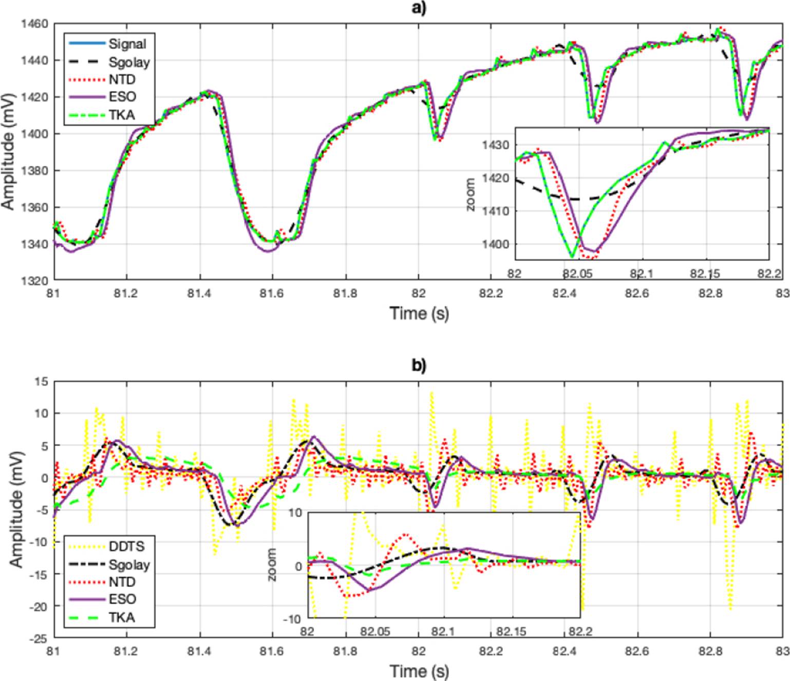
Figure 3 a) Signal reconstruction using the Sgolay, NTD, ESO and TKA methods. b) Zoomed-in view of the estimation. c) Estimation of the derivative of the estimated signal and include the derivative estimation with DDTS. 

In Table 2, the RMSE error (17) estimates in signal and derivative estimate are show, as can be seen, TKA provided the better signal reconstruction. The best derivative estimates of the synthetic signal were obtained by NTD, the estimates in TKA are degraded by the transients, however they are closer to the NTD estimates and can be obtained without an additional derivative stage. The derivative of the synthetic signal is provided by the derivative of each function (f₀(t), f₁(t), … , f₈(t)). However, since the measurement signal does not provide a known derivative, the error is not calculated. To obtain the derivative of the measurement signal, it would need to be processed by another method. Hence, in Table 2, only the error of the signal is calculated.

Table 2 RMSE in signal and derivative estimates. 

Signal		RMSE
		METHOD
		Sgolay	NTD	ESO	DDTS	TKA
Synthetic	Signal	0.0059	0.0311	0.0102	Not applicable	7.2722×10-5
	Derivative	0.1821	0.006	0.0059	0.0061	0.0089
ECG	Signal	12.0219	12.9263	13.7664	Not applicable	7.7915×10-5
RAW	Signal	4.4964	5.6750	7.4522	Not applicable	1.1348×10-5
Blood	Signal	1.5211×10-4	0.2916	0.0577	Not applicable	4.1782×10-15
RAW 2	Signal	0.0475	0.0525	0.0656	Not applicable	1.4625×10-15

As a reference for the accuracy of the estimations, the root mean square error (RMSE) is calculated, which is defined as (Equation 17):

RMSE=∑(sn -s^t )2N (17)

where s(n) represents the input signal and the signal estimation is defined as ŝ(t) and N is the ample size.

CONCLUSIONS

The objective of this work is to verify the efficiency of TKA for the estimation of biomedical signals; three types of biomedical signals (ECG, synthetic ECG, cardiorespiratory and blood pressure) were analyzed. The capacity for signal reconstruction and derivative estimation were compared with the Sgolay, NTD, ESO and DDTS methods. Also, the estimation of the input signal is not obtained by the DDTS method, because it can only estimate the derivative of the signal. The results obtained for signal estimation show an advantage over the Sgolay, NTD and ESO methods, as well as a superiority in the estimation of its first derivative compared to the ESO method. On the other hand, note that the estimation is with respect to the synthetic derivative of the ECG signal, which has large discontinuities. Hence, in measurement signals that are smoother, it could be expected that the estimates in the derivative would have more precision. Looking ahead, to enhance the generalizability of our findings, we plan to extend our testing to include a wider array of real physiological signals like EMG and EEG.