Introduction

Controllability stands as a cornerstone concept within mathematical control theory, constituting a qualitative property essential for understanding dynamical control systems. At its core, controllability signifies the capacity to guide a dynamical system from any starting point to a specified end state utilizing admissible controls. However, it’s worth noting the diverse range of definitions attributed to controllability in the literature. These definitions vary depending on the class of dynamical systems considered and the characteristics of the admissible controls involved ^{[1] [2]}.

Addressing controllability across different dynamical systems demands the application of various mathematical tools and theories. These encompass principles drawn from a variety of mathematical disciplines, such as functional analysis, matrix analysis, differential geometry, topology, ordinary and partial differential equations, and difference equations ^{[3] [4]}. Despite the breadth of methods available, there remain numerous unresolved challenges in controllability analysis, particularly concerning nonlinear types of dynamical systems ^{[1] [5]}.

For instance, much of the existing literature on controllability has predominantly focused on unconstrained controls without delays in either the state variables or the controls themselves. This emphasis underscores the need for further exploration and development of controllability concepts tailored to address more intricate dynamical systems with constrained controls and temporal delays ^[6].

Nonlinear models play in epidemiology a vital role for comprehending the dynamics of disease transmission within populations. By translating biological principles and epidemiological data into mathematical equations, models can simulate the spread of diseases, predict future trends, and evaluate the potential impact of interventions ^{[7] [8] [9] [10]}. Epidemiological models often incorporate factors such as transmission rates, population demographics, immunity levels, and behavioral patterns to capture the complexities of disease transmission. These models can help public health authorities develop effective strategies for disease control and prevention, such as vaccination campaigns, quarantine measures, and social distancing policies ^{[11] [12] [13] [14]}. Additionally, mathematical modeling enables researchers to assess the effectiveness of various intervention strategies under different scenarios, providing valuable insights for decision-making in public health emergencies ^{[11] [13] [14]}.

The SIR model, which stands for Susceptible-Infectious-Recovered, is a fundamental mathematical framework used in epidemiology to understand and forecast the dissemination of infectious diseases within populations. In this model, the individuals are classified into three compartments: (S) susceptible, (I) infectious, and (R) recovered. Susceptible persons (S) are those who are at risk of contracting the disease but have not been infected yet. Infectious individuals (I) are those who are presently infected and capable of transmitting the disease to susceptible individuals. Recovered individuals (R) are those who have recovered from the infection and gained immunity, thus they cannot be infected again and do not contribute to disease transmission ^{[15] [16] [17] [18]}.

The dynamics of the SIR model are governed by a system of ordinary differential equations (ODEs) that describe how the number of individuals in each compartment changes over time. These equations capture the flow of individuals between compartments based on the rates of infection and recovery. Specifically, susceptible individuals become infected at a rate proportional to the number of susceptible individuals and infectious individuals, while infectious individuals recover at a certain rate.

By solving these differential equations, the SIR model can provide insights into the dynamics of disease spread, such as the peak of the epidemic, the total number of infections, and the effectiveness of interventions such as vaccination or social distancing measures ^[18].

While the basic SIR model assumes certain simplifications and does not account for demographic factors like births and deaths, it remains a valuable tool for understanding the fundamental principles of infectious disease dynamics and informing public health decision-making. Here, we focus on diseases characterized by the SIR model, especially in situations with large populations or limited demographic data availability, which is described by the following set of equations (Equation 1, Equation 2, and Equation 3):

Where β represents the transmission rate, denoting the speed at which susceptible individuals contract the infection upon exposure to infectious individuals, g is the recovery rate, denoting the rate at which infectious persons recover from the disease and become immune. u is the control variable representing the treatment or intervention applied to infectious individuals. N is the population size given by N=S+I+R which is constant.

In many disease control strategies, the primary objective is to minimize the number of infected individuals over time, aiming for the long-term eradication of the disease. However, in certain scenarios, achieving this goal may take an extended period ^[11], rendering it insufficient for immediate containment. In our work, we address this challenge by focusing on the design of a control mechanism that not only aims to reduce the overall number of infections but also ensures that the number of infected individuals falls below a predetermined threshold within a specific desired time-frame. This approach is particularly crucial in situations where rapid containment is necessary to prevent further transmission and mitigate the impact of the disease outbreak.

Materials and methods

Results and discussion

In this section, computational techniques are employed to evaluate the effectiveness and performance of the proposed control strategies within the SIR model, which is solved using the fourth-order Runge-Kutta method. Using numerical simulations, we explore various scenarios and parameters to assess the impact of the control mechanisms on disease dynamics. By simulating the spread of infectious diseases under different conditions, we aim to gain insights into the efficacy of the proposed strategies in containing outbreaks, reducing the number of infections, and achieving predefined control objectives.

In these simulations, our population consists of N=25150 individuals, with S₀ =25000 initially susceptible, I₀=150 initially infected, and R₀=0 initially recovered individuals. The transmission rate is set to β=0.41 (Rate of new infections per day) and the recovery rate to g=0.005 (Rate of recoveries per day). All parameters chosen for these simulations are intended as academic examples. The primary goal in choosing these values was to depict a significant peak of infection, allowing a comprehensive comparison of outcomes with and without control measures.

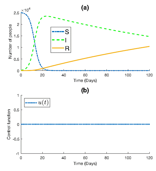
Figure 1 depicts the progression of the epidemic within the population. We observe a peak in the number of infections, reaching approximately 2.4×10⁴ individuals before gradually declining to around 1.5×10⁴ by the end of the simulation. Concurrently, the number of susceptible individuals experiences a sharp decrease, approaching zero around t=30 in the simulation. Conversely, the number of recovered individuals exhibits a slow but steady increase, reaching approximately 10⁴ by the simulation’s conclusion.

Figure 1 (a) S, I and R functions. (b) The control function u. 

The decline in infections coincides with a significant decrease in the number of susceptible individuals, indicating the depletion of the susceptible population due to infection.

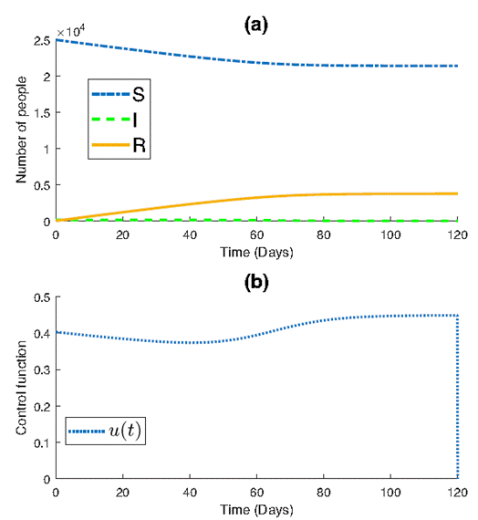
After using the proposed control (4) with a=1.3522×10³ and ϵ = 0.1, it can be seen in Figure 2b that despite 𝜖 not satisfying the conditions outlined in theorem (1), the control remains admissible, where , and .

Figure 2 (a) S, I and R functions. (b) The control function u. 

Figure 2a illustrates the impact of implementing the control law on epidemic dynamics. Notably, the control strategy effectively reduces the number of infected individuals compared to the scenario without control. A gradual and stable decline in the number of susceptible individuals is observed, converging to approximately 2×10⁴ by the end of the simulation. This contrasts with the rapid decline observed in the absence of control measures.

Additionally, the number of removed individuals exhibits a slow but steady increase, reaching approximately 0.4×10⁴ by the end of the simulation. This contrasts with the scenario without control, where a larger number of individuals are removed due to the uncontrolled spread of the disease.

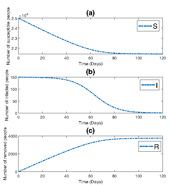
In Figure 3, three subplots are presented, each providing insight into the dynamics of the epidemic. Figure 3a illustrates the evolution of the susceptible population, while Figure 3b depicts the progression of the infected population. Figure 3c showcases the trend of the removed population over time. Figure 3 enables a clearer understanding of each population’s dynamics on different scales. Specifically, smaller numbers, such as the initial infections starting at 150 and gradually declining towards zero, are more easily discernible.

Figure 3 (a) Susceptible, (b) Infected, (c) Removed individuals. 

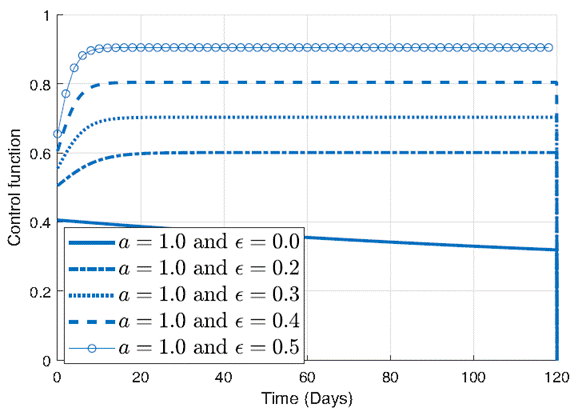
In the Figure 4, the control function is plotted for different values of ϵ, in order to underscore the pivotal role of the parameter ϵ in shaping the behavior of the control function and highlights its significance in designing effective strategies to mitigate the impact of infectious diseases. It can be seen in figure 4 the effect of the parameter ϵ on the control function when a is held constant at 1. Each curve in the plot corresponds to a different value of ϵ, ranging from larger values to smaller ones. As ϵ changes, the control function undergoes noticeable changes in its shape and magnitude.

Figure 4 The impact of Parameter ϵ on the Control Function. 

For larger values of ϵ, the control function exhibits relatively higher amplitude, indicative of a more aggressive intervention approach. However, as ϵ decreases, the amplitude of the control function diminishes, reflecting a milder intervention strategy. Notably, for very small values of ϵ, such as 0.001, the control function demonstrates a significant decrease, suggesting a minimal intervention effort.

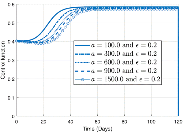
The Figure 5 is presented to highlight the sensitivity of the control function to variations in the parameter a and emphasize the significance of meticulously selecting parameter values to optimize the effectiveness of intervention strategies in combating infectious diseases. Figure 5 presents the influence of the parameter a on the control function where ϵ is set to 0.2. Each curve in the plot corresponds to a different value of a, ranging from smaller to larger values. Notably, all curves exhibit the same shape, demonstrating that the general form of the control function remains consistent across varying values of a.

Figure 5 The impact of a on the control function. 

However, closer examination reveals notable differences in the behavior of the control function as a varies. For smaller values of a, such as 100 or 300, the control function demonstrates a rapid increase, indicating a swift implementation of intervention measures to curb the spread of infection. In contrast, for larger values of a, such as 600, 900, or 1500, there is a noticeable delay in the rate of increase of the control function. This delay suggests a slower response to the increasing number of infections, potentially leading to a longer duration before reaching peak intervention levels.

When comparing the effects of ϵ and a on the control function, it becomes apparent that small variations in ϵ lead to significant changes in the control strategy. Even subtle adjustments in ϵ result in noticeable alterations in the shape and magnitude of the control function, highlighting the sensitivity of the intervention approach to this parameter. Conversely, when considering the parameter a, it becomes evident that larger differences between values are required to observe discernible changes in the control function. Unlike ϵ, where small values induce notable shifts in the control, variations in a necessitate much greater disparities to elicit observable differences in the behavior of the intervention strategy. This implies that the system exhibits lower sensitivity to the parameter a compared to ϵ, with substantial differences needed in a to produce discernible changes in the control function.

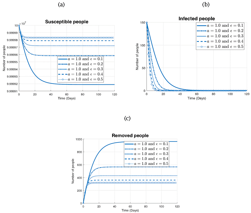
In the three subplots presented in Figure 6, the impact of varying the parameter ϵ on the different states of the model is observed: susceptible (S), infected (I), and removed (R) individuals.

Figure 6 The impact of ϵ on (a) Susceptible (b) Infected (c) Removed people. 

In Figure 6a depicting the susceptibles, it can be seen that as ϵ decreases from 0.5 to 0.1, the rate of decrease in the number of susceptibles accelerates. While in Figure 6b that represents the infected population, we observe the opposite trend. As ϵ increases from 0.1 to 0.5, the rate of decrease in the number of infected individuals becomes more pronounced. This finding is consistent with the dynamics of infectious diseases, where higher values of ϵ indicate a faster recovery or removal of infected individuals from the population. Finally, in Figure 6c illustrating the removed individuals, we observe that all curves exhibit a similar increasing trend over time. However, for larger values of ϵ (0.5 and 0.4), the curve stabilizes around 300 individuals, indicating a slower accumulation of removed individuals. In contrast, for smaller values of ϵ (0.3, 0.2, and 0.1), the curve continues to rise steadily, eventually stabilizing at a higher value of around 950 individuals. This difference suggests that lower values of ϵ lead to a more prolonged period of recovery or removal, resulting in a higher overall number of removed individuals by the end of the simulation.

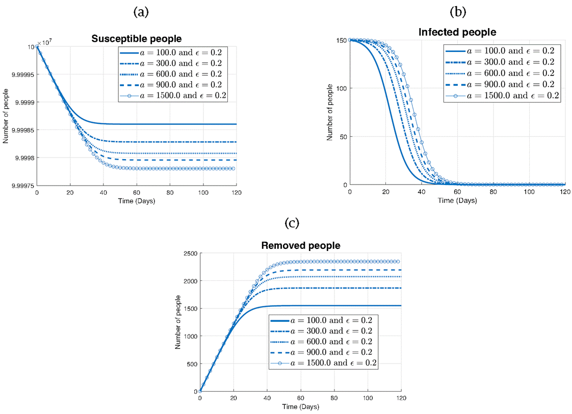
Figure 7 examines the impact of varying the parameter a on the different states of the model: susceptible (S), infected (I), and removed (R) individuals.

Figure 7 The impact of a on (a) Susceptible (b) Infected (c) Removed people. 

In Figure 7a illustrating the susceptibles, it can be seen that as the parameter a increases from 100 to 1500, the rate of decrease in the number of susceptibles accelerates.

While in Figure 7b representing the infected population, it noticed that regardless of the value of a, all curves exhibit a similar shape. However, as a increases, the rate of decrease in the number of infected individuals slows down. This finding suggests that while higher values of a may still effectively control the spread of the disease, they may lead to a longer duration of infection within the population.

Finally, in Figure 7c depicting the removed individuals, it can be seen that all curves follow a similar increasing trend over time. However, for smaller values of a (100 and 300), the curve stabilizes around 1600 individuals, indicating a slower accumulation of removed individuals. Conversely, for larger values of a (600, 900, and 1500), the curve continues to rise steadily, eventually stabilizing at a higher value of around 2300 individuals by the end of the simulation.

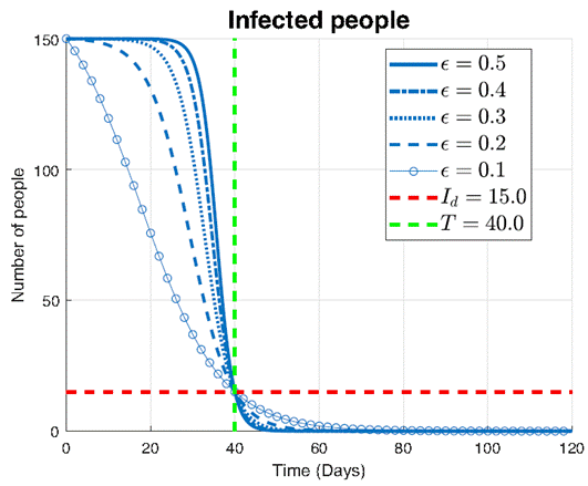
In Figure 8, the impact of different values of the parameter ϵ on the infection dynamics is explored, with a fixed threshold I_d =15 and predefined time T=40. Each curve represents the evolution of the infected population I over time, ranging from ϵ=0.1 to ϵ=0.5.

Figure 8 The impact of ϵ on the controllability effectiveness. 

The key observation from this plot is the efficacy of the proposed control approach in containing the infection within the desired threshold. Across all curves, it can be seen that the number of infections falls below the threshold I_d =15 precisely at the predefined time T=40. This shows the precise controllability achieved by the proposed intervention, regardless of the specific value of ϵ.

However, we notice differences in the shapes of the decreasing curves for varying values of ϵ. For smaller values of ϵ, such as ϵ=0.1 and ϵ=0.2, the infection decreases rapidly. This rapid decline suggests that smaller perturbations in the control parameter ϵ lead to more pronounced effects on infection containment. In contrast, for larger values of ϵ, such as ϵ=0.4 and ϵ=0.5, the infection decreases at a slower rate. This slower decline indicates that larger values of ϵ result in less effective control measures, requiring more time to begin decreasing towards the predefined threshold.

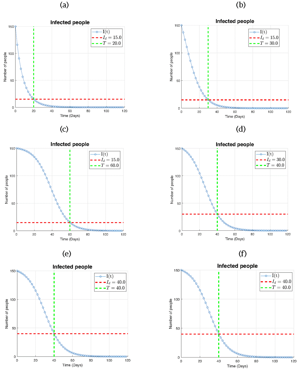
In Figure 9, six subplots are presented illustrating the infection dynamics (I) for various combinations of the threshold I_d and the predefined time T. Each subplot corresponds to a specific pair of values (I_d in individuals and T is time unit) : (a) I_d =15 and T=20, (b) Id=15 and T=30, (c) I_d =15 and T=60, (d) I_d =30 and T=40, (e) I_d =40 and T=40, and (f) I_d =50 and T=40.

Figure 9 The controllability effectiveness. 

Across all subplots, it can be seen that the number of infected individuals precisely reaches the desired threshold I_d exactly at the designated time T. This outcome underscores the remarkable effectiveness of our proposed control law in managing the rate of infection spread within the population.

In Figure 9a where I_d =15 and T=20, we observe the infection curve intersecting the threshold line at T=20, indicating successful containment of the infection within the desired time. Subsequent subplots (b) and (c) exhibit similar trends, with the infection curve intersecting the threshold line at the designated times T=30 and T= 60, respectively.

In Figure 9 (d), (e), and (f), scenarios with higher threshold values of I_d are explored, while maintaining T=40. Despite the varying threshold levels, it can be observed that the infection curve intersecting the threshold line at the predefined time T=40, highlighting the robustness of our control strategy across different infection severity levels.

Figure 10 explores the influence of varying initial infected populations (I₀) on the effectiveness of the controllability. Through three subplots representing the susceptible (a), infected (b), and removed (c) populations, we investigate the impact of different initial conditions on the trajectory of the epidemic, where I_d =40, T=40, S₀ =10⁸ and R₀=0

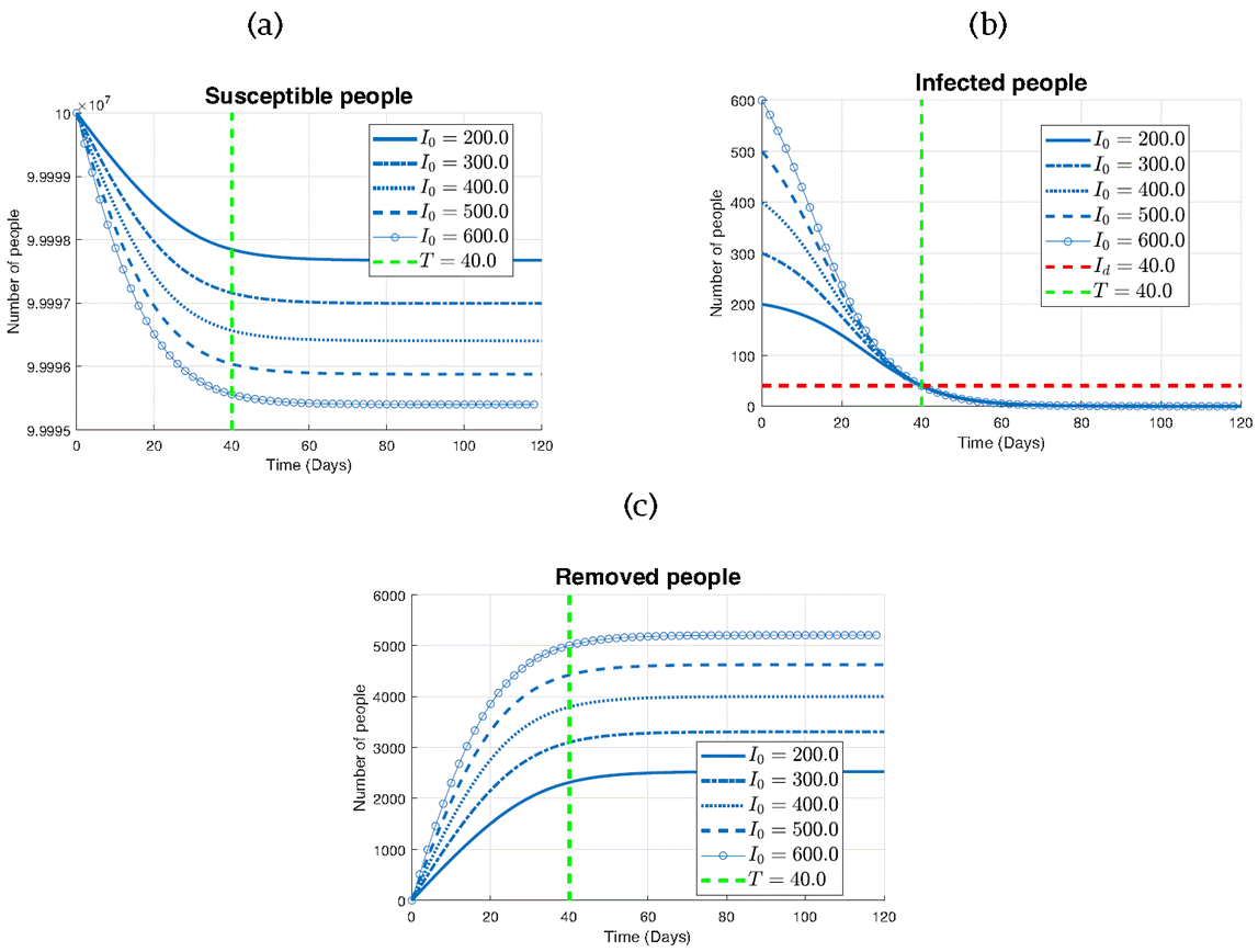
Figure 10 The impact of I₀ on the controllability effectiveness (a) Susceptible individuals, (b) Infected individuals and (c) Removed individuals. 

Firstly, focusing on the infected population (Figure 10b), it can be observed that all curves intersect the predefined threshold line (I_d) at the designated time (T), indicating the successful implementation of the control strategy. This demonstrates the ability of the control measures to achieve the desired containment objective regardless of the initial outbreak size.

For the susceptible population (Figure 10a), we note a discernible trend: for larger initial infected populations (I₀), the decline in susceptible individuals is more pronounced. This suggests that higher levels of infection exert greater pressure on the susceptible population, leading to a more rapid depletion of susceptible individuals.

In contrast, when examining the removed population (Figure 10c), a contrasting pattern is observed. Here, larger initial infected populations result in a more substantial increase in removed individuals over time. This observation highlights the effectiveness of the control strategy in transitioning infected individuals to the removed category.

When the initial infected population is large, there is a higher probability of interactions between infected and susceptible individuals, resulting in increased transmission of the disease.

Consequently, more individuals become infected over time. However, with the implementation of effective control measures, such as vaccination campaigns, quarantine measures, or other interventions, the transmission dynamics are disrupted.

The impact of varying the initial values of S₀ and R₀ on the effectiveness of controllability is also investigated. However, it found that regardless of the initial values of S₀, the function I showed no changes. Similarly, variations in the initial values of R₀ did not affect the dynamics of the infection. These observations suggest that the controllability of the system remains robust and relatively unaffected by changes in the initial states of susceptible and recovered individuals.

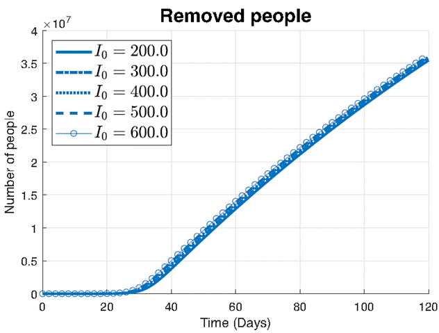
Figure 11 investigates the impact of varying initial values of infected individuals (I₀) in the absence of control measures where S₀ = 10⁸ and R₀ = 0. Through this analysis, it was observed that without control, there is a substantial increase in the number of removed individuals, indicating the natural progression of the infection. Conversely, when implementing control measures, such as those outlined in Figure 10cc, the number of infections remains relatively low, resulting in a smaller number of individuals transitioning to the removed category. This clear contrast underscores the effectiveness of the control strategy in mitigating the spread of infection and minimizing the number of individuals affected.

Figure 11 Impact of I₀ on removed people without the control. 

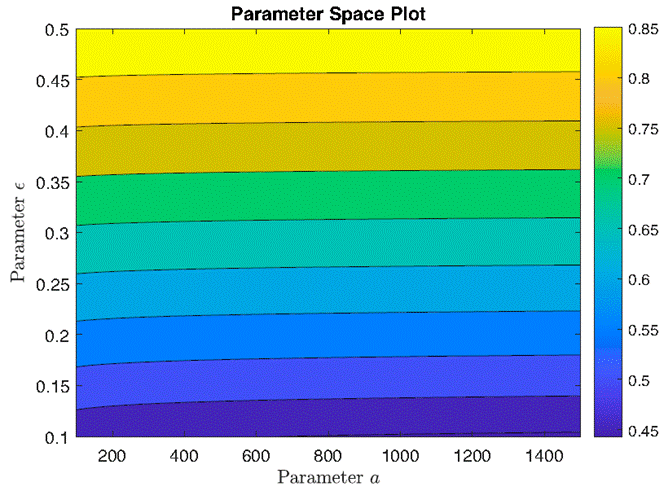
Figure 12 illustrates a parameter space analysis of the maximum intensity of the control function u(t) across varying combinations of parameters a and ϵ. Each point in the parameter space grid represents a unique combination of parameter values. The color intensity represents the maximum value of the control function achieved for each parameter combination. This analysis provides insights into how changes in parameters a and ϵ influence the effectiveness of the control strategy. This figure illustrates the admissibility the control for a wide range of parameters.

Figure 12 Impact of I₀ on removed people without the control. 

Our proposed control strategy, tailored for the SIR model, offers distinct advantages over existing approaches ^{[22] [23] [24]}. While these papers provide valuable insights into controlling infectious diseases and focus on generic control methods, our proposed control stands out in terms of precision and adaptability.

One key advantage of our proposed control is its ability to ensure the total controllability of the number of infections. The infection dynamics can be guided to a desired state from any initial condition, at a desired time. This level of precision is unparalleled and represents a significant advancement in epidemic control strategies. In contrast to the methods discussed in ^{[22] [23] [24]}, which rely on Pontryagin's principle to reduce the number of infections, our approach offers greater control over the infection dynamics. While Pontryagin's principle is effective in minimizing infections, it lacks the precision and flexibility inherent in our proposed control strategy.

Conclusions

This study addresses the formidable challenge of controllability in nonlinear models, with a specific focus on designing a control strategy to manage infection dynamics within the SIR framework. By tackling this complex task, our research contributes significantly to the field of epidemiology, offering policymakers and public health authorities invaluable insights for implementing targeted interventions and resource allocation strategies.

Our novel control law, tailored specifically for SIR models, represents a significant advancement in infectious disease control.

By providing explicit solutions to the model, our approach effectively mitigates the spread of infection and guides the number of infected individuals towards predetermined thresholds at specified times.

This precision in controlling infection dynamics is essential for effective epidemic management and containment efforts. Through comprehensive numerical simulations, the remarkable efficacy of our proposed control law is depicted. The results unequivocally show that our approach enables precise regulation of the pace of infection decline, aligning with predefined targets with remarkable accuracy. For instance, by employing the proposed control function, a gradual decrease in the infection rate is ensured, ultimately leading it towards zero. Moreover, the approach guarantees that the number of infections will dip below a predetermined threshold at a specified time. This level of precision represents a novel contribution compared to existing studies in the field ^{[22] [23] [24] [25] [26]}, where control functions primarily focus on minimizing the number of infections using Pontryagin's maximum principle.

In ^[22], the authors presented a model for the transmission dynamics of influenza and considered two optimal control strategies involving preventive measures (such as awareness campaigns, hand washing, using hand sanitizer, and wearing masks) and treatment. These strategies were used to minimize the total number of infected individuals and the associated costs of implementing these controls. The objective function was designed to reduce both the infection rate and the cost of interventions. The optimal control analysis and numerical simulations revealed that these interventions effectively reduced the number of exposed and infected individuals.

Similarly, in ^[24], within the framework of a basic susceptible-infected-removed (SIR) model, an Erlang distribution for the infectious period was considered, and optimal isolation strategies were explored. The objective functional to be minimized included the cost of isolation efforts per time unit and the sanitary costs due to the incidence of the epidemic outbreak. The simulations demonstrated that the shape of the optimal solutions was influenced by different distributions of the infectious period, the relative weight of the two cost components, and the initial conditions.

These control strategies did not ensure the convergence of the number of infected individuals to zero. Additionally, they did not provide a mechanism for precisely steering the number of infections toward a predetermined threshold at a specific time, as proposed by our control strategy. Our approach not only aims to reduce the number of infections but also ensures that the number of infected individuals reaches a specific target at a designated time, providing a more precise and effective method of controlling the spread of the infection.

During the early stages of the COVID-19 pandemic, many countries implemented stringent control measures, such as closing borders and enforcing lockdowns, to curb the spread of the virus ^[26]. These measures aimed primarily at reducing the infection rate within a specific time frame, often without considering the significant economic impacts. Such control measures effectively reduced the number of new infections by limiting cross-border movement and preventing the importation of new cases. However, these measures also resulted in considerable economic disruptions, affecting trade, tourism, and overall economic activity.

Our control strategy represents a severe control approach that prioritizes the reduction of infections within a predetermined time frame without any constraints. This strategy is highly effective in significantly reducing the number of infections within the predetermined time 𝑇.

However, while the optimal control methods provided by Pontryagin's Maximum Principle are still effective in reducing infections ^{[22] [23] [24] [26]}, they lack precision in terms of controlling the exact timing and magnitude of infection reduction. The optimal control strategy aims to minimize the infections while simultaneously considering other factors, such as economic costs and social impacts, by incorporating constraints within the objective function. As a result, the optimal control can achieve infection reduction but may not provide precise control over the specific timeframe or the exact number of infections reduced.

This finding highlights the versatility and adaptability of our control strategy, positioning it as a promising tool for epidemic management across diverse settings and scenarios.

Author contributions

O. Z. Conceptualization, formal analysis, writing original draft. S. B. Methodology, formal analysis, and writing review and editing. M. R. Supervision, validation, and writing review and editing.