




 nueva página del texto (beta)
 Inglés (pdf)
 Artículo en XML
 Referencias del artículo
 Traducción automática
 Enviar artículo por email
 Citado por SciELO
  Similares en
SciELO
Similares en
SciELO 
 Permalink
1. Introduction
Venus is the second rocky planet from the Sun (0.72 AU). Its atmosphere is a mixture of gases with 96.5% carbon dioxide (CO2), 3.5% molecular nitrogen (N2), 0.015% sulfur dioxide (SO2), 0.007% argon (Ar), ~0.002% water vapor (H2O), and other chemical compounds in smaller amounts. This mixture gives a molecular weight of 43.44 g mol-1, close to that of CO2. Venus has the most massive atmosphere among the terrestrial planets in the Solar System, exerting a surface pressure of 9.2 × 10⁶ Pa, 91 times greater than that of the Earth’s atmosphere. The surface density and surface average temperature of Venus are 65 kg m-3 and 737 K, respectively (Gulkis and de Pater, 2003; Taylor and Hunten, 2014).
The troposphere of Venus is ~70 km thick and contains 99% of the total atmospheric mass. It also includes a cloud layer between ~48 and 70 km altitude that completely envelopes the planet. It has been established that the clouds were primarily composed of sulfuric acid (H2SO4) droplets, contributing significantly to the planet’s high albedo of 76% (Moroz et al., 1985; Titov et al., 2007; Lebonnois et al., 2010). However, a recent reanalysis of the Pioneer Venus mission datasets, published by Mogul et al. (2025), proposes that cloud aerosols are not predominantly composed of concentrated H2SO4, as previously hypothesized, but rather contain approximately 60% water by mass. This significant water fraction appears to be sequestered within hydrated sulfate salts, likely involving iron and magnesium cations, potentially sourced from meteoric dust.
Venus has a mean radius of a = 6051.3 km, very close to the mean radius of the Earth, and rotates on its axis with an angular velocity Ω = 2.98×10⁻⁷ s-1, two orders of magnitude smaller than that of the Earth. Its rotational period is ~243 Earth days, longer than its orbital period of 224.7 Earth days. Its atmosphere rotates in the same direction as the solid planet, but at cloud level it rotates 60 times faster, with zonal winds reaching speeds exceeding 100 m s-1. This phenomenon is known as superrotation and is one of the most conspicuous phenomena in Venus’ atmosphere that is not yet fully understood (Titov et al., 2007; Sánchez-Lavega et al., 2017).
Similar to Earth, the energy that drives the circulation of Venus’ atmosphere is solar radiation. Consequently, an unresolved issue is to quantitatively explain how radiant energy is transformed into the atmosphere’s mechanical energy, particularly regarding superrotation. In trying to find answers to this problem, researchers have used general circulation models (GCMs) (e.g., Yamamoto and Takahashi, 2003a; Lee et al., 2007; Mendonça and Read, 2016; Takagi et al., 2018; Sugimoto et al., 2019) and have looked at the role that waves and turbulence have in maintaining superrotation (Takagi and Matsuda, 2007; Kouyama et al., 2019).
To give a physically plausible explanation for the maintenance of superrotation, Matsuda (2010) mentions three possible mechanisms based on: (a) the circulation between day and night (diurnal circulation) due to the prolonged insolation that Venus receives during its solar day (Venus day) of ~117 Earth days (Schubert and Whitehead, 1969); (b) momentum transport associated with the vertical propagation of thermal tides excited by solar heating in the cloud layer (Fels and Lindzen, 1974; Takagi and Matsuda, 2007); and (c) meridional circulation and angular momentum transported upward and poleward (Gierasch, 1975; Rossow and Williams, 1979; Matsuda, 1980, 1982).
Takagi and Matsuda (2007) addressed mechanism (b) by means of a GCM where diurnal and semi-diurnal thermal tides excited by solar heating generate and maintain the atmospheric superrotation of Venus through momentum transport; the superrotation extends from the surface up to 80 km altitude with a vertical profile similar to the observations (Fujisawa et al., 2022). The assimilation of data from the Akatsuki orbiter improved the view of the three-dimensional structures of thermal tides and found that they play a crucial role in maintaining the superrotation of the Venusian atmosphere.
Sugimoto et al. (2023) conducted simulations using a Venus atmospheric GCM at medium and high resolutions, exploring a range of horizontal diffusion strengths. They found that fully developed super-rotation could be maintained across a specific range of diffusion values, indicating that its structure is largely independent of horizontal diffusion within that range.
Previous numerical studies with GCMs (Takagi and Matsuda, 2007; Titov et al., 2007; Takagi et al., 2018; Kouyama et al., 2019) have also shown the importance of thermal tides in maintaining the superrotation of Venus’ atmosphere, which plays an important role in the transport of angular momentum balance. For example, Fukuya et al. (2021) found that the semidiurnal tide has a large enough amplitude to contribute significantly to the maintenance of superrotation. Yamamoto and Takahashi (2003b) conducted a study that reproduced significant atmospheric superrotation with zonal velocities exceeding 100 m s-1 at the cloud-top level (~70 km), characterized by a strong meridional circulation in a single cell extending from the surface to approximately 80 km above the clouds. The authors also incorporated a dominant process into their superrotation model, employing the generation mechanism proposed by Gierasch (1975), which involves the angular momentum balance between mean meridional circulation and wave transport (mechanism c) (Matsuda, 2010).
Yamamoto and Takahashi (2007) demonstrated that vertical eddy diffusion plays a crucial role in shaping the dynamics of Venus’ atmosphere, especially in sustaining superrotation. Cohen et al. (2025) employed the Venus Planetary Climate Model and data from the Pioneer Venus probes to identify three distinct atmospheric circulation regimes, each occurring at different altitudes and associated with varying rotation rates.
Regarding thermodynamic models, Takahashi et al. (2024) examined how the radiative-convective equilibrium structure of Venus’ lower atmosphere depends on various atmospheric thermodynamic models. They concluded that employing an ideal gas model with a temperature-dependent specific heat that reproduces the adiabatic lapse rate profile of real gases is a promising approach.
In any case, the actual thermodynamic and dynamic mechanism by which the superrotation of Venus’ atmosphere is generated and maintained is not entirely clear.
The purpose of this work is twofold: (1) to present a simplified global thermodynamic model where the dynamics is subordinated to thermodynamics, and (2) to provide a theoretical explanation of how the horizontal gradients of the geopotential play an important role in establishing and maintaining the global circulation of Venus’ atmosphere, especially the superrotation, due to the differential heating of the solar radiation between day and night (zonal gradient) and between the equator and the poles (meridional gradient).
2. Method and model description
The atmospheric and surface temperatures are computed using conservation of thermal energy applied to the tropospheric and surface regolith layers. The tropospheric layer includes a cloud cover enveloping the entire planet. The equations of atmospheric motion are obtained in pressure coordinates, assuming a constant temperature lapse rate and hydrostatic equilibrium, and using the ideal gas equation; the geopotential can be expressed as a function of the pressure coordinate and the atmospheric temperature at the surface. The regolith surface-layer temperature is obtained using the thermal conductivity equation as a function of the atmospheric surface temperature and the regolith subsurface-layer temperature.
2.1 The tropospheric thermodynamic equation
The tropospheric temperature is obtained by vertically integrating the conservation of thermal energy equation for a column of unit area from the surface to the Venus tropospheric top at ~70 km. The atmosphere includes a planetary cloud cover with a thickness of ~22 km, between 48 and 70 km altitude. The corresponding energy balance can be expressed in a similar way as has been applied to the Earth’s atmosphere (Adem, 1965):
where the superscript (*) indicates variables that depend on altitude
(z), horizontal coordinates, and time; ⟨ ⟩ represents space
and time average values; ('') in the horizontal velocity
vector and in the temperature represents the turbulence and fluctuation of
velocity and temperature with respect to their time-averaged values,
respectively; H is the thickness of the troposphere;
ρ* is the density; c
v
is the specific heat at constant volume; T* is the
temperature; t is the time, V* is the
horizontal wind velocity, and ∇ is the horizontal gradient
operator in two dimensions. The term
To simplify the thermodynamic model, in Eq. (1) we have not considered the transport of thermal energy by horizontal wind and vertical currents; however, we believe that its incorporation can appreciably modify the temperature field, initiating a non-negligible feedback process between thermodynamics and the dynamics of the atmosphere. Additionally, we neglected the vertical turbulent transport of thermal energy at the top of the atmosphere, which includes the rate at which the thermal energy increases due to heat transfer by molecular conduction and friction, and the rate at which the thermal energy increases in the column due to work done by compression on the column. Moreover, Eq. (1) does not include the latent heat released by condensation since we assume that it is used to evaporate the H2SO4 raindrops before they reach the surface.
We further assume that horizontal turbulent heat transport occurs in the opposite direction to the temperature gradient, which can be expressed as:
where K is the turbulent exchange coefficient (Austausch coefficient), which is considered constant.
We consider the troposphere to be an ideal gas in hydrostatic equilibrium with a
constant temperature lapse rate Γ. To have temperature fields
in terms of pressure coordinates, we assume that the acceleration of gravity g
remains constant between the equator and the poles and between the surface and
the top of the troposphere at z = H; then, the
geopotential Φ* can be approximated as Φ* = gz. In this way,
the planet’s average surface at z = 0 results in an
equipotential surface or constant geopotential surface Φ* = 0. Therefore,
assuming a constant temperature lapse rate Γ, the temperature
field
where T s is the surface atmospheric temperature at Φ* = 0 and γ=Γ/g. Assuming an atmosphere in hydrostatic equilibrium and using the equation of state and Eq. (3), the hydrostatic equilibrium equation can be expressed as:
where R is the gas constant. The solution of Eq. (4) is given by:
Eq. (5) expresses the geopotential Φ* (λ, φ, p*, t) as a function of the longitude λ latitude φ and, explicitly, the pressure p* as a vertical coordinate and time t. The temperature T s (λ, φ, t) is only a function of λ, φ and t. In (5) p s is the isobaric surface, which coincides with the surface of Venus, and where, according to (5), the geopotential is zero. From now on, Φ* (λ, φ, p*, t) will be simply expressed as Φ*, the same for the other variables of the model.
Substituting (5) into (3), we obtain the temperature in pressure coordinates:
where
Using Eq. (6),
We substitute Eq. (7) in the integrals of Eq. (1), considering that
H is the altitude of the isobaric surface where the
troposphere ends. Such surface corresponds to p =
3.6×10³
Pa (~70 km). Neglecting the orographic effects, we assume that
Venus’ surface pressure corresponds to p
s
= 9.2 × 10⁶ Pa; in this way, p
m
= 4.6 × 10⁶
Pa (~10.5 km). Therefore, considering the equation of
hydrostatic equilibrium
Here, we used the parameterization from Eq. (2) for the third integral,
neglecting the integral of the turbulent transport term,
where the approximation is due to
2.2 Radiation balance
Assuming that the Venus atmosphere is composed of 96.5% CO2, which is well mixed in the troposphere, we have calculated, as in Mendoza et al. (2017, 2021), the emissivity ϵa of the Venus troposphere using the spectral calculator E-TRANS, with the database HITRAN (Rothman et al, 2009), finding that ϵa = 0.94, which is almost a black body emissivity:
Here, σ is the Boltzmann constant, and
E(T*) is the energy per unit area and time
emitted by the tropospheric horizontal borders, being only a function of the
temperature (for simplicity
We define
where p C = 1.4 × 10⁵ Pa (~48 km) is the lower cloud cover boundary pressure.
Figure 1 shows the model’s radiation balance scheme, similar to that on Earth (Adem, 1962); however, on Venus, the cloud cover is complete, while on Earth it is partial. In this figure, we notice that per unit area and time, the regolith surface absorbs solar radiation α 1 I, the troposphere α 2 I, and the cloud cover α 3 I, with the fractions α 1 , α 2 and α 3 related to the planetary albedo α p through:
where I is the insolation or solar radiation arriving at the planetary surface per unit area and time in the absence of atmosphere, computed with the Milanković formula (Milanković, 1920) using the Venus orbital parameters from Archinal et al (2018). Figure 2 shows the solar radiation I (W m-2) at the beginning of a Venusian day, whose maximum intensity of 2566.5 is centered on longitude 0º E on the equator, advancing in the west-east direction and returning to the same position after ~117 Earth days, when the sunrise is at 90º E.
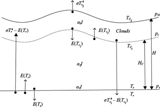
Fig. 1 Representation of the radiation balance of the Venus troposphere with a cloud layer covering the entire planet. In this figure, T r is the surface temperature of regolith.
Following Titov et al. (2007) , we use constant values for α 1 , α 2 and α 3 : α 1 = 0.032, α 2 = 0.048, and α 3 = 0.16, such that using Eq. (12), the planetary albedo is α p = 0.76
According to Figure 1, the radiation balance (the difference between the incoming and outgoing energies) in the troposphere, including the radiation balance in the clouds, is expressed as:
where T r is the surface temperature of the regolith. The radiation balance at the surface E r is:
To linearize E T and E r in Eqs. (13) and (14), we consider a basic temperature T 0 * and its perturbation T*'. The temperature T 0 * is a function of the isobaric coordinate p* obtained from Eq. (7) when T m is replaced by the constant T m0 . Likewise, T*' is obtained from Eq. (7), when T m is replaced by T m ' = T m - T m0 . Taking T* = T 0 * + T*', expanding the function E(T*) in Taylor series and considering that |T m '|/T 0 * << 1, we have:
Then, the linearized form of equations (13) and (14) is:
where T' r = T r - T r0 is the perturbation of T r and T r0 is a constant temperature. The constants F n are:
The constant temperatures
2.3 Thermal energy balance at the upper regolith layer.
The regolith upper layer temperature T r is calculated from the equation of conservation of thermal energy. We assume that in this layer, the stored thermal energy can be neglected; therefore, the heat transfer by net radiation E r , and the vertical turbulent sensible heat transport G 2 given to the atmosphere, are in balance with the heat G 1 transferred by thermal conductivity from the regolith upper layer to the underlying regolith layer. The equation is:
Here, G 1 and G 2 are:
where k
v
is the thermal conductivity coefficient; h
r
is the thickness of the upper regolith layer;
Here:
Substituting T' r from (23) in (16) and (22), we found that the tropospheric heating in Eq. (8) can be expressed as:
where:
The temperature T' g in Eqs. (23) and (25) is calculated using the equation of thermal conductivity in the regolith:
where ρ
r
and c
r
are the density and specific heat of the regolith and T
r
*' is the temperature of each regolith layer. In Eq.
(27), the thermal conductivity coefficient is related to the thermal inertia
I
T
, by
2.4 The equations of motion
To compute the zonal and meridional wind components U* and V*, respectively, where the zonal wind in Venus flow is positive in the westward to eastward direction, and the meridional wind is positive when flows from south towards the north pole, we will use the equations of horizontal motion, with ζ* = -ln(p*/ps) as the vertical coordinate and assuming hydrostatic balance, where (as we mentioned in Eq. [5]), both p* and ps correspond to isobaric surfaces at levels z and z = 0, respectively. These equations are similar to those given by Saltzman (1978):
The vertical component of velocity ω ζ * is computed from the continuity equation:
The vertical component of velocity w* is positive when it flows from the surface to the top of the atmosphere (normal to the surface), where the vertical coordinate z is related to ω ζ * through the hydrostatic equation and the equation of state, resulting in the following approximation:
In Eqs. (28) and (29), the geopotential Φs* is given by Eq. (5); f is the Coriolis parameter; ν is the horizontal turbulent viscosity coefficient, and ε* is the Rayleigh drag coefficient. Furthermore, following the idea of the Rayleigh friction model (Stevens et al., 2002), the zonal and meridional components of the vertical gradient of turbulent stress can be expressed for the troposphere as -ε* U* and -ε*V*, respectively. These terms have the effect of slowing down the horizontal motion of the atmosphere and are thought to originate in the process of thermal convection, vertical turbulence (between 40 and 60 km), weak random eddies in the planetary boundary layer (PBL), and gravity waves excited by mountains (Gierasch, 1975; Schubert et al., 1980; Lefèvre, 2022). We further assume that the efficiency with which vertical turbulence slows horizontal motion depends on atmospheric density. In this way, we propose that:
where we used the ideal gas equation, and ε s and ρ s are the values of ε* and ρ* at the surface. Stevens et al. (2002) use ε s = 2.2 × 10⁻⁵ s-1, and we adjusted this value empirically from the experiments to ε s = 1.5 × 10⁻⁵ s-1.
When the meridional equatorward component of the centrifugal force is in balance with the meridional poleward component of the force due to the geopotential gradient, then the circulation of the atmosphere is in cyclostrophic balance. These components are part of the equation of motion (Eq. [29]), so that the cyclostrophic balance can be expressed as:
In spherical coordinates, the Laplacian in Eqs. (4), (28), and (29) for any continuous scalar function and with continuous derivatives is given by:
2.5 Numerical solutions of the equations
To numerically solve Eqs. (28) and (29), we used the semi-implicit method,
approximating the time derivatives by the corresponding finite differences:
where
Eqs. (35) and (36) can be written as a single equation as follows:
For the case ψ = U* we have:
For the case ψ = V*, F 84 , F 85 and F 89 do not change, while:
Substituting the tropospheric heating E
T
+ G
2
from Eq. (25) in the thermodynamic Eq. (8) and using the approximation
Our method of obtaining the superrotation of the Venusian atmosphere is based on a simplified realistic thermodynamic model, from which we can obtain the geopotential given by Eq. (5) in terms of the atmospheric surface temperature Ts , which can be expressed in terms of Tm, using the first equality in Eq. (11). Temperature Tm is computed from the thermodynamic Eq. (8), where the advection and convection of thermal energy have been neglected; in this way, the complex coupling between the thermodynamic equation and the dynamic equations is excluded from the problem, and consequently, the dynamics are subordinated to the thermodynamic state of the atmosphere.
Eq. (37), for the cases in which corresponds to the wind components U* and V* or
to the temperature T'm, is integrated using finite differences centered
for the space derivatives in a latitude φ between -89.5º and 89.5º, and a
longitude λ between 0.5º and 359.5º; in radians:
The model equations given by Eq. (37) are not applied at the poles, since, in
spherical coordinates, these points can result in singularities. In this way, to
carry out the spatial derivatives of temperature and velocities with respect to
latitude on the borders, defined by the latitude circles close to the poles
({j = 1; i = 1,2,…,360} for the south pole
and {j = 180; i = 1,2,…,360}) for the north
pole, we assign for the grid point at each pole, the average temperature over
the corresponding border, while U*, V* and
Therefore, the derivatives with respect to φ at the boundaries
are:
The thermodynamic model equations are the thermodynamic equation, Eq. (8) for the atmosphere and Eq. (20) for the surface, the thermal conductivity Eq. (27), the movement, Eqs. (28) and (29), and the continuity equation, Eq. (30).
To integrate the thermal conductivity equation, Eq. (27), the regolith is divided
into 24 layers, including the surface layer. The thickness of each layer varies
and is given ∆z = h
r
exp[0.1(n - 1)], with n =
1,2,…,24; then for n = 1, ∆z =
h
r
= 0.20m and for n = 24, ∆z = 1.99 m,
resulting in a thickness of 19.1 m for the complete regolith layer. We employ
centered differences using 1 h time steps for spatial and temporal derivatives.
The border conditions are T
r
*' = T'
r
for the upper layer and
The velocity is computed in 24 levels from the surface ζ* = 0 to the top of the troposphere ζ* = -ln(pH/p s ) = 7.846), these levels are separated from each other by ∆ζ = -ln (pH/p s ) / 24 = 0.327. In this way, using finite differences centered on the vertical, the continuity Eq. (30) can be expressed as:
where k = 1,2,3,...,24 and where we have used the approximation (ω* ζp ) k = [(ω* ζp ) k+1 + (ω*ζp) k-1 ] / 2, assuming that on the surface ω* ζp = 0.
For the vertical momentum transport terms
The vertical velocity w* in z coordinates can be determined in terms of the vertical velocity ω* ζ using the hydrostatic equilibrium equation and the equation of state and Eq. (31).
The initial conditions for the temperature perturbations are T' mp = 0, T*' rp = 0 for each regolith layer, U* p = V* p = 0 and ω* ζp = 0 for the velocities at each ζ* level. First, we integrate the thermal conductivity Eq. (27) using 24-time steps of 1 h to complete one terrestrial day; the temperature T' g obtained in the last time step is used to integrate the thermodynamic Eq. (8), where we use time steps of one Earth day. The computed tropospheric temperature T' m is expressed in terms of T' s using the first equation in Eq. (11) and with Eq. (5) we calculate the potential Φs*; finally, with Eqs. (35) and (36) and the continuity Eq. (38), we calculate the velocity components U* V* and ω* ζ , using 24-time steps of 1 h. With T' m and T' g we calculate T' r using Eq. (21). The next steps are similar, using T' m , U*, V* and T' g computed in the previous time steps as initial conditions in the prognostic equations. The model is integrated for 300 Venus days until the tropospheric temperature, wind, and tropospheric angular momentum are stabilized; this is achieved after ~86 Venusian days (~10 062 Earth days).
3. Data
The atmospheric layer emission spectrum is found from the spectral calculator E-TRANS using the database HITRAN (Rothman et al, 2009), resulting in an emission spectrum close to that of a black body. The surface regolith and the cloud cover are considered black bodies themselves.
Meridional profiles of the zonal wind and the mean north-south wind (m s-1) were obtained from cloud tracking measured at UV wavelengths at an altitude between 65 and 70 km of the Mariner 10 missions, 1974; Pioneer-Venus, 1980, 1982; Galileo, 1990; Venus Express VIRTIS, 2006-2012 and Venus Express VMC, 2006-2012 in the daytime (Sánchez-Lavega et al., 2017).
We also used data from the Venera vertical profiles 8, 9, 10, and 12 and Pioneer-Venus reported by Schubert et al. (1980).
4. Results and discussion
The experiments that comprise this work are three: the baseline experiment (BL experiment), which includes all terms in the equations; the experiment in which the zonal gradient of the geopotential is set to zero (ZGZ experiment); and the experiment in which vertical momentum transport is set to zero (VMTZ experiment).
The surface temperature (K) of the Venusian atmosphere calculated by the model at the
beginning of the 300th Venusian solar day (that is, 34 984 Earth days), when the
maximum insolation is located at 0º E longitude (see Fig. 2), is shown in Figure 3. The
maximum surface heating occurs at the equator, between 75º and 60º W, and advances
behind the maximum insolation. Due to the meridional gradient of insolation, the
temperature difference between the equator and the poles is ~12.0 K. The maximum
surface temperature on the equator is reached just before sunset, while the minimum
is reached shortly after sunrise. This thermal contrast of 12.0 K between the
equator and the pole is considerably greater than that simulated by a GCM, shown in
Figure 1a of Takagi et al. (2018), which is in the order of 1 to 4 K. The
thermal contrast between the equator and the pole at the clouds upper level (~70 km)
can be determined by our model applying Eq. (6) at this level, when
p* = p
H
= 3.6 × 10³ Pa, where the temperature
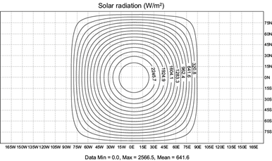
Fig. 2 Insolation or solar radiation at the planetary surface per unit area and time computed with Milanković’s formula in the absence of an atmosphere.
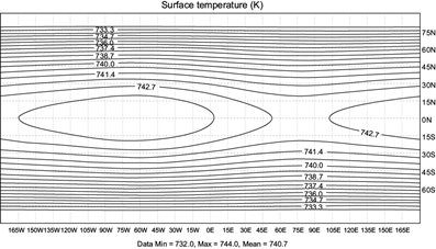
Fig. 3 The Venusian atmosphere’s surface temperature (K) was computed at the beginning of the 300th Venusian day (Earth day 34 984).
For the BL experiment, the computed time series of the surface temperature (K) (in red) and the zonal and meridional components of the wind (m s-1) at ~68.5 km altitude (in blue and purple, respectively) are shown in Figure 4. The model runs for 300 Venusian days (35100 Earth days) to ensure that temperature and wind reach a stable condition, which begins to occur after ~86 Venusian days (10 062 Earth days). The temperature (Fig. 4a) corresponds to the average in the tropical region from 20.5º S to 20.5º N and 173.5 to 185.5º E. In comparison, the wind components (Fig. 4b) correspond to the north latitude region between 24.5 and 73.5º N and between 173.5 and 185.5º E. The last seven Venus days (819 Earth days) of this run are also shown for the temperature and wind components (Fig. 4c). The thermal and dynamic oscillation period is 117 Earth days, which is one Venusian solar day. The tropical temperature oscillation has an amplitude of ~1.4 K, that is, between 743.8 K just before sunset (see Figs. 2 and 3) and 742.4 K at sunrise, while the zonal and meridional wind components oscillate between -80.2 and -102.45 m s-1 (~22 m s-1), and 13.5 and -10.5 m s-1 (~24 m s-1), respectively. The temperature and zonal wind are out of phase by ~48 Earth days, while the temperature and the meridional wind by ~22 days.
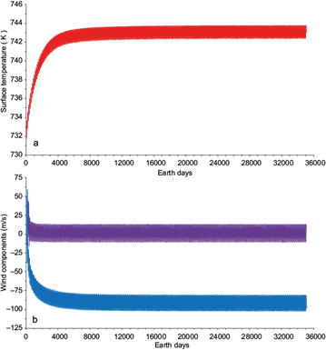
Fig. 4 Modeled time series for 300 Venus solar days. (a) Computed average surface temperature in the tropical region between 20.5º S and 20.5º N, and 173.5 to 185.5º E; (b) computed average zonal and meridional wind components at ~68.5 km of altitude (blue and purple curves, respectively) in the northern region between 24.5 to 73.5º N, and 173.5 to 185.5º E; (c) the last seven Venus days of these series for the temperature and the wind components.
We consider that the radiation balance E T in the troposphere of Venus, given by Eq. (13), which includes the radiation balance of the cloud layer, and the radiation balance E r at the regolith surface, given by Eq. (14), are appropriate since when used in the thermodynamic Eqs. (8) and (20), respectively, they give as a solution a global mean atmospheric temperature at the surface level of 740.7 K (see Fig. 3) with certain agreement with observations (Lorenz et al., 2018). In addition, the oscillations indicate that said temperature remains stable during the 300 Venusian days of the model run (Fig. 4).
If we assume the atmosphere of Venus rotating as a solid body equal to the rotation of the planet, so that its zonal velocity turns out to be equal to a Ωcosφ, then its total angular momentum can be calculated, integrating the density of the angular momentum ρ* (aΩcosφ)acosφ over the entire volume of the atmosphere; the result is (8/3 πa 4 Ωp s )/g = 3.47 × 1027 kgm 2 s-1. On the other hand, the relative angular momentum of the atmosphere M r , associated with the zonal wind U*, is calculated by integrating the angular momentum density ρ* U* acosφ over the entire volume of the atmosphere. According to Golitsyn (1984), the result of this integral is in the range of (3 to 4)×1028 kg m2 s-1. Figure 5 shows the relative angular momentum of the troposphere calculated by our model, whose value 3.2 × 1028 kg m2 s-1 is reached approximately after Venusian day 60. This computed value is within the range of values given by Golitsyn (1984).
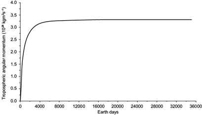
Fig. 5 Relative angular momentum (1028 kg m2 s-1) of the troposphere associated with the zonal wind calculated by the model.
The computed components of the zonal and meridional wind and vertical velocity, as a function of latitude and altitude, are shown in Figure 6. These results show a prograde zonal wind (zonal winds moving in the same direction of the planet’s rotation) throughout the troposphere (Fig. 6a) that increases with altitude and towards the equator until reaching wind speeds greater than 75 m s-1 above 50 km altitude. Near the top of the troposphere (~70 km), a prograde tropical jet (between -20º and 20º latitude) is established with a speed of ~90 m s-1. When comparing the zonal component of the wind simulated by our model (Fig. 6a) with the intercomparison of the eight GCMs in Figure 8.2 of Lebonnois et al. (2013), we find that these models exhibit a significantly different wind pattern compared with the simulation produced by our model, for example, the UCLA high resolution finite volume model simulates only a 50 m s-1 equatorial jet at an altitude of ~70 km (~3.6 × 10³ Pa). As the equatorial air rises (Fig. 6c), it moves towards the poles (Fig. 6b), where it descends (Fig. 6c) after ±20° latitude, suggesting the establishment of a direct thermal circulation (DTC).
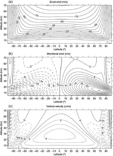
Fig. 6 Computed components of the (a) zonal, (b) meridional, and (c) vertical velocity as a function of latitude and altitude. These velocity components correspond to the average of the last Venusian day. The vertical velocity is computed using Eq. (31).
In the polar regions (between 60 and 70º latitude) at an approximate altitude of 15 km, strong winds develop towards the poles that exceed 28 m s-1. This DTC, which exceeds 10 m s-1 below ~40 km altitude (Fig. 6b), suggests two large asymmetric Hadley cells in both hemispheres whose thickness is greater near the equator, where the air rises, reducing towards the poles, where the air descends. However, the meridional circulation does not show an overturning branch (Fig. 6b), which may be due to the simplification of our model in comparison with the GCMs, which show a more complex meridional circulation with several superposed cells, when these models incorporate a realistic radiative transfer and the topography (Lebonnois et al., 2010).
Gierasch et al. (1997) present a vertical profile of w*, obtained with a simplified model that predicts vertical velocities in the Hadley cells of the order of 10 m s-1. According to Figure 6c, our results show lower values: near the equator, the upward flow, between 35 and 70 km altitude, is ~2 cm s-1; in mid-latitudes (± 45º) it is ~1.0 cm s-1, and close to the poles (± 80º), where there is air subsidence, it is between ~-6.0 cm s-1 at ~70 km altitude, and ~-1.0 cm s-1 near the surface.
A clear prograde zonal flow at cloud level (68.5 km), whose velocity increases from the poles toward the equator, is shown in Figure 7a. During the night (see Fig. 2), two large polar jets are established in both hemispheres (~30 N and ~30 S), heading towards the dayside with wind speeds closer to -100 m s-1 heading towards the equator. These jets are associated with the air descent shown in Figure 7c.
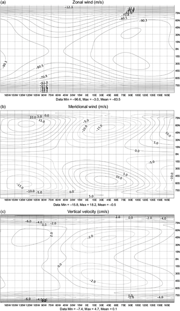
Fig. 7 Velocity components are now shown as a function of latitude and longitude at an altitude of ~68.5 km (5.0 × 10³ Pa). These components correspond to those calculated at the beginning of the last Venusian day (Earth day 48 358): (a) zonal wind (m s-1); (b) meridional wind (m s-1); and (c) vertical velocity (cm s-1).
The model result has a significant discrepancy with observations and high-resolution modeling (e.g., Fujisawa et al., 2022) regarding meridional circulation at the cloud-top level. While previous studies indicate a daytime poleward flow, our scheme produces a flow from the poles to the equator with speeds exceeding 10 m s-1.
This fundamental difference can be attributed to a key simplification in the thermodynamic approach: integrating the thermal energy equation for the entire tropospheric column (Eq. [1]) using a constant lapse rate, rather than performing a level-by-level radiative heating calculation. This approximation, combined with the troposphere’s high thermal inertia, introduces a lag between the instantaneous peak insolation and the resulting peak surface temperature. Since the vertical thermal profile is constant, this surface temperature pattern and its lag are projected to remain unchanged at all levels, including the cloud top (approximately 70 km).
Consequently, the region of maximum atmospheric heating in the model shifts toward the night side. Because the geopotential field-and thus the driving force for the meridional wind-is derived directly from this temperature, the resulting cloud-level circulation is reversed: the equator-to-poles flow occurs at night, and the poles-to-equator flow occurs during the day. This outcome contrasts with mechanisms in which cloud-level heating is predominantly direct and diurnal, generating a circulatory response in phase with the Sun.
It is important to mention that the surface temperature field (Fig. 3) and the planetary waves associated with the velocity components (Fig. 7) move in the same direction as the insolation (Fig. 2), that is, from west to east; however, the direction of the zonal wind associated with the superrotation is in the same direction in which the planet rotates; that is, a prograde zonal wind.
It is interesting to determine the relative importance of the zonal and meridional gradients of the geopotential contribution to the superrotation of the Venusian atmosphere. In this way, Figure 8a, b obtained in the ZGZ experiment (zonal gradient of the geopotential equal to zero), shows that the meridional gradient of the geopotential due to the meridional insolation gradient is sufficient to generate superrotation of the Venusian atmosphere in the dynamic equations.
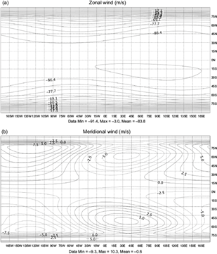
Fig. 8 (a) Zonal and (b) meridional components of the wind (m s-1) at an altitude of ~68.5 km, where we have neglected the zonal gradient of the geopotential; that is, we assumed that ∂Φ*s/∂λ = 0 in Eq. (28).
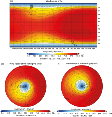
Figure 9, obtained in the BL experiment, shows that in the high-latitude jet region (60º N and 60º S), the circulation is markedly zonal; however, at dawn, there is a meridional movement towards the equator in both hemispheres contributing to the equatorial jet; at sunset (~75º W in Figure 2) the meridional movement changes direction, now heading towards the poles, increasing the speed of the wind by conservation of angular momentum. An asymmetric vortex is established at each pole (b) and (c), with its maximum velocity forming part of the high-latitude jet.
5. Comparison with observations in the BL experiment
Figure 10 shows the meridional profiles of the zonal wind (m s-1) obtained from cloud tracking measured at UV wavelengths at an altitude between 65 and 70 km. The wind profile curves are not shown here but are within the gray area of this figure and are averages from the Mariner 10 missions, 1974; Pioneer-Venus, 1980, 1982; Galileo, 1990; Venus Express VIRTIS, 2006-2012, and Venus Express VMC, 2006-2012 in the daytime. Figure 2 of Sánchez-Lavega et al. (2017) shows these profiles. The black solid curve corresponds to the average made during the hours of sunshine and is calculated using the motion equations (Eqs. [35] and [36]) at the ~68.5 km level. The dotted curve is calculated using cyclostrophic equilibrium (Eq. [33]) at the same level, with the zonally averaged geopotential gradient and the square root multiplied by -1. At an altitude of 68.5 km, we find that the computed meridional profile lies within the range of observed values and is close to the meridional wind profile obtained by cyclostrophic equilibrium. The profile shows an equatorial maximum of ~90 m s-1, which is within the range of observations; however, the two observed mid-latitude maxima in each hemisphere are not reproduced by the model.
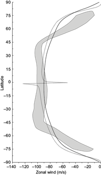
Fig. 10 Meridional profiles of zonal wind (m s-1) obtained from cloud tracking at UV wavelengths during daytime in the altitude range between 65 and 70 km. The profiles, which are not shown here, are present within the gray area. Our model calculates the black solid curve and the dotted curve at ~68.5 km. The solid curve is calculated with the equations of motion (Eqs. [35] and [36]) and corresponds to the average made during the hours of sunshine; the dotted curve is calculated with the cyclostrophic balance (Eq. [33]) using the zonally averaged geopotential gradient and multiplying the square root by -1.
The computed meridional profiles of the global mean north-south wind at this height agree with the dominant direction observed in each hemisphere; that is, negative towards the southern hemisphere and positive towards the northern hemisphere. Its magnitude is only ~3 m s-1, while the observed magnitude is ~10 m s-1. However, at night, when the Sun has warmed the surface, the meridional wind moves from the poles to the equator, and the calculated meridional profile shows greater agreement with the observed profile (Fig. 11).
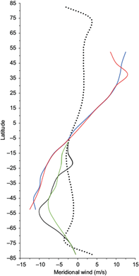
Fig. 11 Meridional profiles of the mean north-south wind as measured at the upper cloud level (65-70 km): Pioneer Venus, 1979-1983 (blue line); Galileo, 1990 (red line); Venus Express VIRTIS, 2006-2012 (black line); Venus Express VMC, 2006-2012 (green line). These curves were obtained from Fig. 5 in Sánchez-Lavega et al. (2017). The global mean meridional profile of the north-south wind at 68.5 km altitude is given as computed by the model (dotted curve).
The global daily average zonal wind profile (Fig. 12) computed by the model is within the range of the corresponding observations. Below the level at which approximately half of the atmospheric mass is contained, the average computed zonal wind is close to zero and becomes relevant above 10 km. At 35 km, the computed wind reaches a speed of ~55 m s-1, and at 70 km, it reaches ~77 m s-1, 42.7 times the rotation velocity of the planet at the equator.
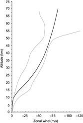
Fig. 12 The shaded area contains the observed vertical profiles of the zonal wind by the Pioneer-Venus and Venera probes 8, 9, 10, and 12. The black curve corresponds to the profile calculated by our model globally averaged on the last Venusian day (day 300).
The angular momentum density profiles obtained from the zonal wind and atmospheric density in the four Pioneer Venus probes (Schubert et al., 1980) are located within the gray area of Figure 13. The Sounder probe near the equator and the Day and Night probes in tropical latitudes show a maximum at 20 km altitude, which is reflected in the right edge of the shaded area while the North probe at high latitudes shows a maximum at ~25 km altitude. The model profile (solid black curve), which is a global average of the last Venusian day (day 300), has a maximum at ~23 km altitude. This figure shows that above 70 km altitude, the contribution of the angular momentum density to the computed relative angular momentum Mr of the entire atmosphere can be neglected, which explains why the value we obtain for Mr of 3.2 × 1028 kg m2 s-1 in the troposphere is within the range given by Golitsyn (1984). The comparison in Figure 13 between the solid curve and the dashed curve obtained from the experiment VMTZ, suggests that the vertical transport of specific momentum in the motion equation (Eqs. [28] and [29]), plays an important role in maintaining the zonal circulation between the surface and the cloud base at ~48 km altitude, overcoming vertical turbulent friction with the surface. Above the cloud base, superrotation is maintained mainly by the force associated with the meridional gradient of the geopotential, even without a specific moment’s vertical contribution.
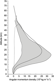
Fig. 13 Angular momentum density ρ* U*
acosφ (108 kgm-1 s-1) as a function of
height. The gray area contains the profiles obtained from zonal wind and
atmospheric density measurements by the four Pioneer Venus probes. The
solid black curve is obtained from the zonal wind and atmospheric
density computed by the model. The dashed curve corresponds to the VMTZ
experiment where the vertical transport terms of specific momentum
6. Discussion: thermal gradients as primary forcing in the context of superrotation theories
Our results identify horizontal temperature gradients-derived from a thermodynamic model-as the principal forcing factor for superrotation in slowly rotating planets, offering a perspective that complements and synthesizes several mechanisms proposed in the literature.
Traditionally, explanations for superrotation on Venus and Titan have focused on momentum-transport mechanisms driven by waves (gravity, tidal, or Rossby waves) and turbulence, which balance the meridional flow (Read and Lebonnois, 2018). Our work does not contradict these mechanisms but proposes a more fundamental origin for momentum injection: direct thermal forcing. In essence, day-night and equator-pole gradients, sustained by high thermal inertia and slow rotation, generate a robust ageostrophic circulation in cyclostrophic balance. This idea connects directly to the work of Peng and Mitchell (2014), who demonstrated that an ageostrophic instability, fed by such gradients, can be an efficient engine for accelerating zonal winds to superrotating states without the need for topographic forcing.
This approach also sheds light on the apparent rarity of robust superrotation among the solar system’s planets. The key lies in the unique dynamical regime created by slow rotation. As Laraia and Schneider (2015) insightfully discuss in a broader context, the transition to a superrotating state is favored when the planetary rotational constraint is weak. Crucially, this corresponds to a large Rossby number regime. Venus, with its exceedingly long sidereal day, epitomizes this regime. Here, inertial and advective forces dominate the Coriolis force, allowing significant deviations from geostrophic balance and facilitating the organization of flow by large-scale thermal gradients rather than by rotation.
Our thermodynamic model directly quantifies the second essential ingredient in this weak-rotation regime: thermal forcing. A large Rossby number is necessary but not sufficient. Superrotation also requires that radiative processes permit the establishment of large-scale, sustained horizontal temperature gradients. On a rapidly rotating planet like Earth, the strong Coriolis force efficiently organizes such thermal contrasts into geostrophically balanced mid-latitude jets, suppressing the mean meridional overturning needed for superrotation. In contrast, on a slow rotator like Venus, the weak rotational constraint allows intense diurnal and hemispheric heating contrasts-calculated by our model-to drive a powerful, direct thermal circulation. This ageostrophic flow, operating in a high-Rossby-number environment, becomes the primary agent for the upward and poleward transport of angular momentum.
We refined the paradigm: the superrotation regime arises from the confluence of a weak rotational constraint (high Rossby number) and powerful, sustained thermal gradients. Our work provides the thermodynamic basis for this second condition, showing that Venus’ combination of an exceptionally long solar day (~117 Earth days), which drives meridional and day-night heating contrasts, and high thermal inertia creates the necessary thermal forcing. This forcing then acts through ageostrophic dynamics-either through a direct mean circulation or through instabilities, as in Peng and Mitchell (2014)-to accelerate the zonal flow, which is subsequently shaped and maintained by wave-driven processes (Read and Lebonnois, 2018).
Thus, we situate our findings within a unifying framework: in slowly rotating bodies, meridional and diurnal thermal gradients-thermodynamically computed by our model-act as the primary forcing that initiates and sustains superrotation, while wave and mixing mechanisms provide the necessary coupling and redistribution to establish and maintain the global atmospheric jet.
7. Summary and conclusions
Seventy-six percent of the solar radiation that reaches Venus’ atmosphere is reflected into space mainly by the cloud layer. Only 24% penetrates the atmosphere, where most of it is absorbed by the clouds (16%), followed by the atmosphere (4.8%) and a small part by the surface of the regolith (3.2%); however, the heavy atmosphere of the planet, constituted mainly by CO2, behaves almost like a black body for longwave radiation, so that in thermodynamic equilibrium, the surface temperature reaches the average value of ~745 K (472 ºC), being this the most prominent solution of the model.
The main mechanism of heat transport in the Venusian troposphere in our model is horizontal, planetary-scale eddy turbulent heat transport, which mainly smooths the meridional temperature gradient. After performing several sensitivity experiments, we found that the turbulent exchange coefficient required in our solution is equal to 4.5 × 10⁵ m2 s-1, one order of magnitude lower than that used for the Earth’s troposphere (Schubert et al., 1980). The incorporation of thermal energy advection is an important component of the energy budget that contributes to the smoothing and redistribution of the meridional temperature gradient, which can improve the results.
We have assumed a constant lapse rate in the troposphere in hydrostatic equilibrium; therefore, using the equation of state, we have expressed the geopotential as a function of pressure (a vertical coordinate) and the atmospheric temperature field at the surface (Eq. [5]). The result means that the geopotential increases with height, starting from zero at the surface, where p s = 9.2 × 10⁶ Pa, and reaching a typical value of 6.21 × 10⁵ m2 s-2 (computed with T s 0 = 737 K) at the top of the troposphere, where p = 3.6 × 10³ Pa. The gradient of the geopotential increases the acceleration of the specific momentum with height. A steady state is achieved at each level due to the balance between the gradient of the geopotential, the vertical turbulent stress in the PBL, and the divergence of the horizontal turbulent transport of momentum. This transport occurs against the momentum gradient, which is parameterized in the model using a viscosity coefficient (ν = 1.2 × 10⁷ m2 s-1).
Above 10 km altitude, the average zonal wind exceeds the rotation velocity of the planet at the equator (superrotation). According to Figure 6a, at the upper level of the clouds, the superrotation of the zonal wind manifests with a prograde zonal wind of ~85 km s-1 in lower latitudes. The vertical transport of specific momentum in the equations of motion plays an essential role in maintaining the zonal circulation between the surface and the cloud base at ~48 km altitude, overcoming vertical turbulent friction at the surface. Above the cloud base, superrotation is maintained mainly by the force associated with the meridional gradient of the geopotential, even without the vertical transport contribution of a specific moment. In this way, the theoretical solution of the equations of motion predicts the position and intensity of mid-latitude prograde jets (35º N and 35º S) between the day and night side at ~90º E. These mid-latitude jets are present in the meridional profile of the observed zonal wind in Figure 10.
Thermal tides are fluctuations in the temperature field that occur in response to solar heating near the equator. These fluctuations manifest as waves in the thermal field that propagate vertically and horizontally through the atmosphere, transporting heat from warm to relatively cold regions, redistributing thermal energy, and smoothing its gradients. According to Horinouchi et al. (2020), thermal tides help balance heat transfer and angular momentum redistribution, stabilizing and maintaining superrotation at the cloud level.
The agreement of our results with the observations leads us to conclude that the diurnal thermal tide associated with the west-east advance of solar heating at the surface, manifested in the temperature field T s and consequently in the zonal and meridional gradients of the geopotential, is the main force that generates and maintains the superrotation of the atmosphere.
It is not necessary to perform a radiative-convective adjustment process in the model because the lapse rate is prescribed to be constant throughout the troposphere. In a radiative-convective adjustment process, vertical heat transfer by thermal tides may also play an important role. In our model the constant lapse rate determines the vertical profile of the geopotential by being part of the coefficient (1 γ-1) and the exponent (Rγ) in Eq. (5), consequently the advance of solar heating at the surface, associated with the diurnal thermal tide, is also manifested at the cloud level, establishing the superrotation at that level. However, Fukuya et al. (2021) found that semidiurnal tides are predominant around cloud tops, while our results are dominated by diurnal tides at this level.
As a final remark, the essential aspect of our thermodynamic model consists in the fact that the dynamic part of the superrotation of the atmosphere of Venus is subordinated to the temperature field, that is, the solution of the equations of conservation of thermal energy in the atmosphere and the surface of the regolith.
Data availability
The thermodynamic model of Venus code and results are available in https://zenodo.org/records/8432706 (Mendoza et al., 2024).
Figures 2, 3, 7, 8, and 9 were made with Panoply v. 5.4 developed by NASA Goddard Institute for Space Studies, available at https://www.giss.nasa.gov/tools/panoply/download/.

