




 nueva página del texto (beta)
 Inglés (pdf)
 Artículo en XML
 Referencias del artículo
 Traducción automática
 Enviar artículo por email
 Citado por SciELO
  Similares en
SciELO
Similares en
SciELO 
 Permalink
1. Introduction
Accurate air quality forecasting is essential for protecting human health and guiding environmental policy, particularly in densely populated megaregions where pollution episodes can have significant public health impacts. Central Mexico, home to over 30 million inhabitants, encompasses Mexico City and the six surrounding states (seven jurisdictions in total), collectively known as the Megalopolis region. These states face persistent challenges from ozone (O3) and particulate matter (PM) pollution (SEDEMA, 2024). Meteorological drivers, complex topography, and diverse emission sources-ranging from mobile to industrial and residential sectors-contribute to episodic high-ozone events that exceed both national and World Health Organization standards (SEDEMA, 2018; WHO, 2021).
Over the past decade, numerical modeling tools such as the Weather Research and Forecasting model coupled with Chemistry (WRF-Chem) have become increasingly vital for operational air quality forecasting in urban and regional environments (Grell and Baklanov, 2011). WRF-Chem allows for interactive simulation of meteorological and chemical processes, enabling forecasts of surface-level pollutant concentrations on hourly time scales (Zhou et al., 2017). Successful applications in regions analogous to Central Mexico include the operational forecasting system developed by the Secretaría del Medio Ambiente de la Ciudad de México (Ministry of the Environment of Mexico City, SEDEMA), which provides a one-day forecast focusing only on the Mexico City Metropolitan Area (MCMA) and is based on WRF-CMAQ. Worldwide, there are operational air quality forecasting systems for ozone and particulate matter (Guevara et al., 2017). For instance, studies in Houston (Nam et al., 2006; Tie et al., 2007), India (Beig et al., 2021), and Chile (Saide et al., 2016) have shown that improved emissions inventories and data assimilation markedly enhanced ozone prediction accuracy. However, uncertainties in emission inventories, chemical initial and boundary conditions, and model parameterizations can lead to degraded skill, particularly beyond 24 h (Grell and Baklanov, 2011; Zhou et al., 2017).
In Mexico, the 2016 National Emissions Inventory provides a comprehensive but coarse-resolution basis for numerical simulations. Spatial and temporal disaggregation of this inventory-using models such as DiETE-provides an improved representation of volatile organic compounds (VOCs) and nitrogen oxides (NOₓ), critical precursors of ozone formation (García-Reynoso et al., 2018). Nevertheless, even high-resolution inventories require continuous validation and adjustment against observational data from monitoring networks to ensure reliability in operational contexts (Eder et al., 2006; Beig et al., 2018; SEMARNAT, 2020; Tsikerdekis et al., 2024; Vallejo et al., 2025).
This study builds on prior efforts at the Institute of Atmospheric Sciences and Climate Change (ICAyCC) of the National Autonomous University of Mexico (UNAM) to develop an operational forecasting system tailored for Central Mexico based on WRF-Chem (García et al., 2016). It is important to note that, apart from SEDEMA, the only other operational air-quality forecasting system in Mexico is the one developed at UNAM. To the authors’ knowledge, these two are the only systems currently operating for Mexico City. To date, more research is needed to develop a national-level operational forecast that can assist urban and rural areas that lack both computational and monitoring infrastructure.
This paper is organized as follows. Section 2 presents the description of the forecasting system. The proposed evaluation procedure is presented in section 3. The main findings are presented in section 4 and discussed in Section 5. Finally, section 6 summarizes the conclusions and future work.
2.Description of the forecasting system
An operational air quality forecasting system has been developed and implemented at the Institute of the ICAyCC-UNAM to provide daily predictions of pollutant concentrations (Rodríguez and García, 2021). The main region of interest is the megalopolis of Central Mexico, which includes Mexico City and the six surrounding states (seven jurisdictions in total). This area is one of the most densely populated and industrially active regions in Latin America.
The forecasting system is based on WRF-Chem, a community-supported modeling tool that can interactively simulate meteorological and chemical processes (Grell et al., 2005). The model is driven by meteorological inputs from the Global Forecast System (GFS) with a spatial resolution of 0.25° (NCEI, 2015). The model-ready emission files employ a chemically speciated, temporally disaggregated emissions inventory derived from the Mexican 2016 Emissions Inventory and were generated with the DiETE model (García-Reynoso et al., 2018). The system is designed to produce a daily forecast up to three days (72 h) in advance.
The configuration employs a single modeling domain of 90 × 90 grid cells at approximately 3 km horizontal resolution using a Lambert Conformal projection. It has a spatial extent of 270 km. The lateral boundaries have a five-cell relaxation width. The vertical structure includes 34 atmospheric levels. The physics configuration follows the “Tropical” suite, except for the convective parameterization, which uses the Grell 3D (cu_physics = 5), an improved version of the Grell-Devenyi (GD) ensemble scheme. Grell 3D convective parameterization was selected because: (1) it smooths the transition between a parametrization scheme and explicit resolution; (2) it represents subgrid vertical transport; and (3) it improves the vertical distribution of moisture, heat, and pollutants in air quality models. Previous studies showed that application of adaptive schemes in this spatial resolution rang, (Grell and Freitas, 2014; Prein et al., 2015). Four-dimensional data assimilation is enabled (grid_fdda = 1) with a 180-min nudging interval. Grid nudging is applied to keep consistency with synoptic information. Previous studies have shown that using weak nudging, or restricting it above the PBL, can improve regional transport without degrading model performance (Stauffer and Seaman, 1994; Otte, 2008; Gilliam et al., 2012). In this study, we restricted nudging of the U, V, T, and q fields outside the PBL and above 10 vertical levels using the prescribed nudging coefficient (3E-4).
Regarding chemistry and emissions options, the model setup includes the NOAA/ESRL RACM Chemistry (Goliff et al., 2013) with MADE/VBS aerosols using the KPP (Damian et al., 2002) library (chem_opt = 108), enabling dry deposition of gases and aerosols (gas_drydep_opt = 1 and aer_drydep_opt = 1), vertical mixing of chemical species (vertmix_onoff = 1), and transport through deep convection (chem_conv_tr = 1). Wet scavenging and in-cloud chemistry are both turned off (wetscav_onoff = 0 and cldchem_onoff = 0). The prescribed initial and lateral boundary conditions are based on the global idealized profile included in WRF-Chem, which is derived from the NOAA-Aeronomy Laboratory Regional Oxidation Model (NALROM) (Liu et al., 1996). Short-lived species are initialized to steady-state equilibrium. After the first forecast day was obtained, the chemistry is cycled using ozone, precursors, and intermediate species fields from the previous day’s simulation. After several days (about two weeks), both lateral and initial conditions reasonably well represent the chemical fields in the study region.
Model-ready anthropogenic emissions are disaggregated across the first eight vertical layers to more accurately represent the influence of surface-based sources. Specifically, the emissions from point sources are distributed among the first eight model levels based on effective height calculations using the reported physical characteristics in the National Emissions Inventory.
The primary output variable is surface-level ozone concentration, expressed in parts per billion (ppb), along with other criteria pollutants (NO2, CO, SO2). The forecast products consist of 72-hourly ozone concentration fields starting at 18:00 local standard time (LST) on the day prior to the forecast and ending at 18:00 LST on the third forecast day. These forecasts provide spatially continuous data fields suitable for visual inspection and quantitative validation against monitoring data. In this study, we focus on the period from April 14 to July 2, 2025.
Several key improvements have been incorporated into the operational configuration of the forecasting system to enhance its accuracy and temporal continuity. First, the use of forecasted pollutant concentrations from the previous day as initial conditions has replaced the standard WRF-Chem default boundary fields. This cycling of the chemistry introduces better consistency in atmospheric chemical fields and better alignment with evolving pollution events through frequent warm starts. Second, the 2016 emissions inventory was updated using a non-parametric scaling method based on model-observation comparisons during recent ozone pollution episodes, as described by Rodríguez-Zas and García-Reynoso (2021), who recalibrated the 2013 Mexico Emissions Inventory through scaling factors derived from statistical comparisons between modeled and observed ozone levels, and subsequently validating the revised inventory against March 14-17, 2016 and May 15-21, 2017 ozone episodes. They first scale nitrogen oxides, followed by carbon monoxide, and then VOCs. In this work, the scaling factor for VOC emissions was approximately seven. Previous studies focusing on the MCMA showed that bottom-up inventories underestimated VOC’s effective emissions by a factor of three, and that the simulations are sensitive to their magnitude and speciation (West et al., 2004; Lei et al., 2007). Although the scaling factor is spatially and temporally uniform, the final scaling depends on population, industry type, and the number of vehicles, as reported in the Mexican Emissions Inventory. The associated systematic error may suggest both missing and underestimated emission sources. For example, emissions estimates may underestimate emissions from solvent use and product consumption, leakages of Liquefied Petroleum Gas (LPG), evaporative emissions, and poorly characterized peri-urban emissions such as wildfires (Mendoza-Campos et al., 2015).
This refinement significantly improved the emissions’ spatial and temporal representation, particularly for VOCs, which play a crucial role in ozone formation. Additionally, a new temporal profile was introduced to account for Sunday-specific emission dynamics, which differ notably from weekdays due to changes in human activity and traffic patterns; in this case, the Saturday temporal profile was used for Sunday.
To ensure robust performance evaluation, a dedicated validation framework has been developed. This framework enables continuous comparison of model outputs with observations from Mexico City’s Automatic Atmospheric Monitoring Network (RAMA), focusing on metrics that assess the model’s ability to capture peak pollution levels. It incorporates a set of Python, bash automation, and visualization scripts. The model evaluation has shown that the updated system achieves improved correlation with observed data, particularly in high-ozone episodes, laying the groundwork for more advanced forecasting strategies, including ensemble modeling and real-time data assimilation.
3. Validation methodology
The updated air quality forecasting system evaluation was carried out using a strategy designed to more accurately represent population exposure to peak pollutant concentrations in urban areas. In contrast to traditional methods that rely on point-by-point comparisons between modeled and observed values at individual monitoring stations, this approach compares the maximum hourly ozone concentration forecasted within a predefined urban zone with the maximum value recorded at RAMA monitoring stations in the same area of Mexico City (see Fig. 1). Notably, some monitoring stations that are classified as background stations-typically not considered in contingency alerts-were excluded to ensure the evaluation reflects conditions relevant to public health advisories. The reason for using the daily regional maximum within the MCMA is to represent a similar value to the worst-case exposure used in public health studies (EPA, 2019). The aim is to estimate the highest possible concentration at which the population might be exposed. In Mexico, this highest concentration is used to declare an environmental contingency by the environmental authority, regardless of the monitoring station where it occurred (SEDEMA, 2019).
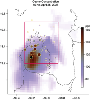
Fig. 1 Hourly ozone concentration forecast (shaded contours, in ppb) for 15:00 LST on April 25, 2025. Observed ozone values from the RAMA monitoring stations are represented as filled circles, scaled by concentration. The red rectangle depicts the area used to evaluate the maximum hourly concentration. (RAMA: Red Automática de Monitoreo Atmosférico.)
The validation domain covers a subregion of the MCMA representative of high ozone concentrations and captures the spatial variability of hourly concentrations. For each 24-h forecast, the maximum hourly ozone value from the domain is compared with the maximum observed value at RAMA stations during the same period.
A set of statistical metrics for dichotomous forecasts was used to quantify the model performance in forecasting events with hourly ozone concentrations above 135 ppb. This threshold is defined by Mexican regulations (SEMARNAT, 2024) as the criterion for “very poor” air quality.
These metrics include the Percent Correct (PC), Probability of Detection (POD), False Alarm Rate (FAR), Critical Success Index (CSI), and the Heidke Skill Score (HSS), among others (CAWCR, 2017; Tsikerdekis et al., 2024). They assess the balance between correct detections and false alarms, and the overall skill relative to a random forecast. This procedure provides a solid basis for assessing the system’s operational capacity and guiding future improvements. The confidence interval for each metric was obtained using a bootstrap approach.
4. Results
The implementation of the updated forecasting system demonstrated notable improvements in predicting high-ozone events across a 72-h forecasting period. Performance metrics were analyzed for each forecast day to assess temporal degradation and detect reliability patterns.
Figure 2 shows the maximum ozone time series before integrating updated emissions, temporal profiles, and initial conditions. The forecasted ozone concentrations (red) remain consistently below 115 ppb throughout the period. On Wednesday (March 12), the difference between forecasted and observed values is 39 ppb. During the initial 10 h of each forecast cycle, the model exhibits low ozone levels due to its initialization with default background concentrations. This underestimation is particularly pronounced on Sunday (March 16), where the modeled ozone concentrations are 84 ppb lower than observations. This highlights the model’s limitation in reproducing weekend ozone dynamics.
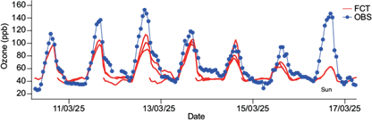
Fig. 2 Time series of observed (OBS, blue) and forecasted (FCT, red) ozone concentrations (ppb) from March 11 to 17, 2025.
Figure 3 shows the time series of maximum ozone concentration after updating the model-ready emissions, weekend temporal profile, and cycling initial conditions. In contrast to previous forecasts (Fig. 2), the forecasted maximum ozone concentrations reach about 155 ppb, closely matching the observed peaks. During the initial 10 h of each forecast cycle, the model successfully reproduces the general trend of observed ozone levels, indicating improved initialization. Notably, on Sunday (April 27), the model better reproduces higher ozone concentrations. The difference is around 26 ppb, which is more consistent with observations and reflects an improved representation of weekend photochemical and emission conditions, particularly in the late afternoon.
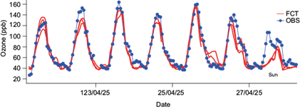
Fig. 3 Time series of observed (OBS, blue) and forecasted (FCT, red) ozone concentrations (ppb) from April 22 to 27, 2025.
Table I shows that performance metrics for Days 1 to 3 reflect a consistent but gradually declining skill in predicting ozone exceedances. Based on the statistical results, the ozone forecast system shows a moderate ability to capture exceedance events, with better performance observed on Day 1. The POD remains relatively high across all days, about 0.76 (IC95%: 0.57-0.94) on Day 1, 0.71 (0.50-0.90) on Day 2, and 0.67 (0.44-0.86) on Day 3, indicating that most true exceedances were identified. However, both the False Alarm Ratio (FAR) and the Probability of False Detection (POFD) increase from Day 1 to Days 2 and 3. FAR rises from 0.47 (0.28-0.65) to 0.60 (0.42-0.76) and 0.59 (0.42-0.75), while POFD increases from 0.23 (0.13-0.35) on Day 1 to 0.37 (0.24-0.49) and 0.33 (0.21-0.46) on Days 2 and 3, respectively. These trends indicate reduced forecast performance with longer lead times, primarily due to a higher number of false positives. The Gilbert Skill Score (GSS), which adjusts for random chance and provides a conservative measure of forecast quality, remains relatively low across all days: 0.31 (0.14-0.48) on Day 1, and 0.16 (0.03-0.31) on both Day 2 and Day 3. This contrasts with the high POD values, suggesting a trade-off between sensitivity and precision in forecast performance. The high POD indicates that the model effectively captures most actual exceedance events (i.e., high sensitivity), but the high FAR and POFD suggest that many of those detections are related to false alarms. Since the GSS penalizes both missed events and false positives, and also adjusts for hits expected by chance, its lower values indicate that part of the correct forecasts may not represent true skill. Therefore, the combination of high POD and low GSS indicates that the forecast system tends to overpredict exceedances, especially as lead time increases. The scatter plot in Figure 4 depicts this tendency to overestimate high concentrations for Day 2 (gray triangles) and Day 3 (blue squares).
Table I Quantitative performance metrics when ozone levels exceed 135 ppb during the period April 14 to July 2, 2025. Metrics include Percent Correct (PC), Probability of Detection (POD), False Alarm Ratio (FAR), Success Ratio (SR), True Skill Statistic (TSS), Critical Success Index (CSI), Heidke Skill Score (HSS), Gilbert Skill Score (GSS), and Probability of False Detection (POFD).
| Metric | Day 1 | Day 2 | Day 3 | ||||||
| MEAN | STD | IC95% | MEAN | STD | IC95% | MEAN | STD | IC95% | |
| PC | 0.77 | 0.05 | (0.66, 0.85) | 0.65 | 0.05 | (0.54, 0.75) | 0.67 | 0.05 | (0.55, 0.76) |
| POD | 0.76 | 0.09 | (0.57, 0.94) | 0.71 | 0.11 | (0.5, 0.9) | 0.67 | 0.11 | (0.44, 0.86) |
| FAR | 0.47 | 0.09 | (0.28, 0.65) | 0.6 | 0.09 | (0.42, 0.76) | 0.59 | 0.09 | (0.42, 0.75) |
| SR | 0.53 | 0.09 | (0.34, 0.71) | 0.4 | 0.09 | (0.23, 0.57) | 0.41 | 0.09 | (0.24, 0.57) |
| TSS | 0.53 | 0.11 | (0.29, 0.73) | 0.35 | 0.12 | (0.1, 0.58) | 0.33 | 0.12 | (0.07, 0.56) |
| CSI | 0.46 | 0.08 | (0.29, 0.62) | 0.35 | 0.08 | (0.2, 0.5) | 0.34 | 0.07 | (0.19, 0.48) |
| HSS | 0.46 | 0.10 | (0.25, 0.64) | 0.28 | 0.10 | (0.07, 0.47) | 0.27 | 0.11 | (0.05, 0.47) |
| GSS | 0.31 | 0.09 | (0.14, 0.48) | 0.16 | 0.07 | (0.03, 0.31) | 0.16 | 0.07 | (0.03, 0.31) |
| POFD | 0.23 | 0.06 | (0.13, 0.35) | 0.37 | 0.06 | (0.24, 0.49) | 0.33 | 0.06 | (0.21, 0.46) |
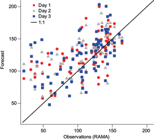
Fig. 4 Scatter plot of observed and modeled daily maxima ozone concentrations (ppb) for Day 1 (red), Day 2 (gray), and Day 3 (blue) in 2025. (RAMA: Red Automática de Monitoreo Atmosférico.)
Compared with the previous year’s forecast performance, the current system shows clear improvement in detecting ozone exceedances. In the earlier version, although the Percent Correct (PC) was 0.74 across all three days-suggesting agreement partly by chance-the system failed to identify any exceedances, as reflected by a POD of 0.00 and a Success Ratio (SR) of 0.00. The skill scores, True Skill Statistic (TSS), HSS, CSI, and GSS, were also zero, indicating that the predictive performance is not better than random classification. The scatter plot in Figure 5 shows the significant underestimation of daily maximum ozone concentrations in the earlier version.
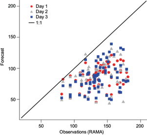
Fig. 5 Scatter plot of observed and modeled daily maxima ozone concentrations (ppb) for Day 1 (red), Day 2 (gray), and Day 3 (blue) in 2024. (RAMA: Red Automática de Monitoreo Atmosférico.)
In contrast, the updated forecast system demonstrates substantial gains in POD, skill scores, and event detection, particularly on Day 1, highlighting significant progress in the model’s capacity to anticipate high ozone events and reduce false negatives.
To complement the categorical analysis, continuous statistical metrics were obtained for the ozone forecast. As with the categorical metrics, a bootstrap approach was used to estimate confidence intervals (see Table SI in the supplementary material). The Mean Absolute Error (MAE) gradually increases from 25.95 ppb (95% CI: 21.07-30.81) on Day 1 to 28.15 ppb (23.02-34.08) on Day 3, while the Root Mean Square Error (RMSE) follows a similar pattern, increasing from 33.88 ppb (28.54-38.86) to 37.07 ppb (29.76-44.65). This confirms a degradation in numerical forecast precision with lead time. However, the bias remains relatively stable with 15.80 ppb (9.14-21.96) on Day 1, 17.79 ppb (11.33-24.24) on Day 2, and 15.74 ppb (8.67-23.11) on Day 3, which indicates an overestimation in ozone concentrations.
Overall, the system shows reasonable performance on the first forecasted day, with noticeable skill deterioration by days two and three. These results suggest that updates to cycling initial conditions and improvements in VOC emissions benefit mostly short-term forecasting up to one day in advance, while highlighting the need for further refinement to reduce overestimation of ozone maxima, which in turn will reduce false alarms and improve discrimination skill beyond 24 h.
5. Discussion
The results demonstrate the value of targeted updates to the forecasting system, particularly for short-term (24-h) air quality predictions. The use of previous-day chemical fields as initial conditions helped preserve continuity in chemical transport, improving both magnitude and timing of peak ozone events. Updates to VOC model-ready emissions, along with refinements for weekend activity, were key in correcting biases in ozone amplitude, especially in urban areas where anthropogenic sources dominate (Crippa et al., 2021). The application of the scaling factor is justified for three primary reasons. First, a temporal update is required because the 2016 emissions inventory is projected forward to 2025, necessitating growth-adjusted emission estimates. Second, the factor compensates for systematic biases: meteorological overestimation of wind speeds over urban areas (Yu et al., 2021) artificially enhances pollutant dilution, and the model’s grid-resolution limitation (3 × 3 × 0.02 km) fails to account for buildings exceeding 20 m in height, thereby reducing the effective mixing volume in street canyons (Gavidia et al., 2021; Kim et al., 2018; Voordeckers et al., 2021). And third, unquantified uncertainty in emission inventories (Solazzo et al., 2021), particularly the absence of confidence intervals, prevents robust sensitivity analysis of baseline emissions.
However, the forecast performance degradation after the first forecasted day highlights the challenge of maintaining accuracy as forecast lead time increases. This degradation is related to known limitations in meteorological predictability and accumulated uncertainties in emissions, photochemistry, and transport (Liu et al., 2023).
The increases in FAR and POFD after the first forecasted day indicate that while the system remains sensitive to potential exceedance events, it tends to overestimate their occurrence. This results in diminished credibility of public alerts. Refining model physics, especially boundary-layer and microphysics parameterizations, and tightening constraints on emissions inputs, particularly those from the mobile sector, could help reduce these false positives.
Despite these limitations, the observed TSS, HSS, and GSS on the first forecasted day suggest relatively good skill in reproducing high and low ozone events. While the Day 1 forecast performs well overall, as shown by TSS and HSS, the GSS highlights areas for improvement in balancing detection and false alarms. This reinforces the value of the forecasting system for public health advisories and policy responses for short-range applications.
Looking forward, integrating ensemble modeling, real-time data assimilation, and use of urbanized models (Steward and Oke, 2012) could further enhance system robustness. Such efforts would enable better quantification of forecast uncertainty and support probabilistic decision-making frameworks in air quality management.
6. Limitations
This study presents the advances in the operational implementation of a 72-h numerical ozone forecasting system for Central Mexico. Even though the regional ozone daily maximum is reasonably well estimated in the first 24 h, the current configuration may be limiting its skill in the last 48 h. For instance, model performance might improve when using nested domains or lateral chemical boundary conditions (Tang et al., 2007, 2021; Pendlebury et al., 2018). However, in this study, a single domain covering the Megalopolis region was used because of limited computational and storage resources. Since the modeled concentration can be influenced by lateral boundary conditions and synoptic forcing at the regional level, the evolution of secondary species such as ozone might be affected, biasing the estimated concentrations and underestimating long-range transport events.
In addition, although wet scavenging of ozone is less efficient at reducing ozone concentrations than for particulate matter, it may nevertheless impact the ozone budget by removing soluble precursors such as formaldehyde and peroxides. This can affect both the magnitude and timing of photochemical production (Niatthijsen et al., 1997; Tost et al., 2007; Ryu et al., 2019). Thus, excluding aqueous chemistry will bias the estimation of the ozone maximum in this configuration, resulting in reduced model performance during the rainy season.
7. Conclusions
The updated operational air quality forecast system developed for the Central Mexico metropolitan area demonstrates substantial improvements in predicting ozone concentrations, particularly for short-term forecasts.
7.1 Future work
To continue improving forecast reliability and operational value, several areas of development are proposed:
Urban influence: Account for interstitial building volumes in air quality modeling, as they directly modulate emission-derived pollutant concentrations, and application of an urban model in operational forecasting to enhance wind intensity predictions in the boundary layer.
Improved emission inventories: Continue refining spatial, temporal, and speciation inputs, particularly for high-impact sectors and weekends, and employ the updated emissions inventory upon its release by the authorities.
Data assimilation: Integrate near real-time meteorological observations and chemical composition data to correct initial conditions and improve forecast accuracy.
Ensemble forecasting: Implement ensemble simulations to characterize forecast uncertainty and provide probabilistic guidance.
User-centered products: Develop tailored forecast visualizations and alerts that address the needs of different user groups, including decision-makers and the public.
These advancements will support the broader application and relevance of the forecasting system for both policy evaluation and operational air quality management in the Megalopolis of Central Mexico.

