Articles
The influence of rainfall on the extinction coefficient and the meteorological optical range

-
Publication dates-
June 24, 2025
April , 2025
- Article in PDF
- Article in XML
- Automatic translation
- Send this article by e-mail
- Share this article +
ABSTRACT
The meteorological optical range (MOR) is an objective parameter for assessing atmospheric visibility. Data collected using optical disdrometers (PWS100) were used to analyze MOR estimates when extreme rainfalls occurred at two locations in Mexico: Chamela, on the Pacific coast, and Juriquilla, a continental sampling site. The performance of the disdrometer for rainfall estimation was found to be consistent and satisfactory when compared to rain gauges. Analyses based on rainfall rate (R) outcomes from tipping bucket rain gauge data showed that MOR measurements registered the most significant decreases during periods of highest R. The assessed coefficients for the extinction coefficient (σ) and R power-adjusted relationships are comparable to those obtained in previous studies, and the statistical performance of the fitted equations in modeling σ values is excellent. The equation coefficients for these mathematical expressions indicate that precipitation at the sampling sites is initiated from mixed (Bergeron-type) clouds, and it can be inferred that mixed-phase thunderstorms were predominant at the sampling sites during the chosen periods. Our findings indicate that MOR and σ are closely related to the large raindrop proliferation and the broadening of the raindrop size distribution (inferred from the increase of the median volume diameter). Despite the underestimation of small raindrops by the optical disdrometer, this study demonstrates the reliability of MOR estimates obtained with the PWS100 during rainfall events.
Keywords::
atmospheric visibility, PWS100, heavy rainfall, Mexico, statistical performance evaluation
1. Introduction
Visibility estimates are based on the contrast between an object and the background, i.e., the relative difference between the brightness of both objects (Koschmieder, 1924; Middleton, 1957). Atmospheric visibility, known as the visual range, is the standard parameter for human visual perception of the environment (Liaw et al., 2009; WMO, 2014) and is an important weather element for safety in ground transportation, navigation, and aviation (Ma et al., 2018; Liu et al., 2022; Zhang et al., 2022).
-
Koschmieder, 1924Theorie der horizontalen sichweiteBeiträge zur Physik der Atmosphäre, 1924
-
Middleton, 1957Vision through the atmosphereGeophysik II/Geophysics II. Handbuch der Physik/Encyclopedia of physics, 1957
-
Liaw et al., 2009Atmospheric visibility monitoring using digital image analysis techniquesComputer analysis of images and patterns, 2009
-
WMO, 2014Guide to meteorological observing and information distribution systems for aviation weather services. WMO-No. 731, 2014
-
Ma et al., 2018The scattering effects on the visibility measurements of laser transmissometer in rain and fogOptik, 2018
-
Liu et al., 2022Visibility classification and influencing-factors analysis of airport: A deep learning approachAtmospheric Environment, 2022
-
Zhang et al., 2022A new method for calculating average visibility from the relationship between extinction coefficient and visibilityAtmospheric Measurement Techniques, 2022
Visibility observations are affected by subjective and physical factors (EPA, 1979). Thus, an objective parameter called meteorological optical range (MOR) has been defined as the path length in the atmosphere over which the light from a known source is reduced to 0.05 of its original intensity (Dunlop, 2008). Heavy precipitation, fog, and clouds lead to reductions in visibility (Gultepe et al., 2019; ICAO, 2005), although emissions and other air molecules can also affect light attenuation and visibility (EPA, 1979). Impaired visibility resulting from heavy rain causes serious problems for highway safety. Records show that crash and injury rates increase by 10 and 8% during rainfall, respectively, and may deteriorate with heavier precipitation due to poor visibility and reduced friction from slippery road conditions (Lee et al. 2018; Wang et al., 2021). Atmospheric visibility is related to light attenuation, expressed by the optical extinction coefficient, σ (in m-1), as the sum of the absorption and scattering effects of particles in the atmosphere (Eidels-Dubovoi, 2002; Duthon et al., 2019).
-
EPA, 1979Protecting Visibility. An EPA report to Congress. EPA/450-5-79-008, 1979
-
Dunlop, 2008A dictionary of weather, 2008
-
Gultepe et al., 2019A review of high impact weather for aviation meteorologyPure and Applied Geophysics, 2019
-
ICAO, 2005Manual of runway visual range observing and reporting practices. Doc 9328 AN/908, 2005
-
EPA, 1979Protecting Visibility. An EPA report to Congress. EPA/450-5-79-008, 1979
-
Lee et al. 2018Traffic accident severity analysis with rain-related factors using structural equation modeling-A case study of Seoul CityAccident Analysis and Prevention, 2018
-
Wang et al., 2021Coupling impacts of spray and rainfall on road visibility and vehicle speeds: A simulation-based analysisCanadian Journal of Civil Engineering, 2021
-
Eidels-Dubovoi, 2002Aerosol impacts on visible light extinction in the atmosphere of Mexico CityScience of The Total Environment, 2002
-
Duthon et al., 2019Light transmission in fog: The influence of wavelength on the extinction coefficientApplied Sciences, 2019
Many empirical relationships between any remote measurable parameter, P, and rainfall rate, R, can have a power-law form (Torres et al., 1994). The literature provides many examples of power-law expressions, among others, between R and radar reflectivity (Atlas, 1964), between rainfall kinetic energy and rainfall momentum (Brodie and Rosewell, 2007; Montero-Martínez, 2021), and between optical extinction coefficient (Atlas, 1953; Ulbrich and Atlas, 1985) and visibility (Gultepe and Milbrandt, 2010). Various instruments are available to obtain visibility (MOR or runway visual range) data, but only those based on transmissometers and forward-scatter meters are currently recommended. Forward-scatter meters have gradually been popularized to replace traditional transmissometers due to several advantages, such as easy installation, minor maintenance, and lower expenses. A series of comparative tests of these two types of devices has been conducted both outdoors and indoors to evaluate their performance (Zhuang et al., 2022).
-
Torres et al., 1994A general formulation for raindrop size distributionJournal of Applied Meteorology and Climatology, 1994
-
Atlas, 1964Advances in radar meteorologyAdvances in Geophysics, 1964
-
Brodie and Rosewell, 2007Theoretical relationships between rainfall intensity and kinetic energy variants associated with stormwater particle washoffJournal of Hydrology, 2007
-
Montero-Martínez, 2021Study of rain classification and the tendency of gamma DSD parameterizations in MexicoAtmospheric Research, 2021
-
Atlas, 1953Optical extinction by rainfallJournal of the Atmospheric Sciences, 1953
-
Ulbrich and Atlas, 1985Extinction of visible and infrared radiation in rain: Comparison of theory and experimentJournal of Atmospheric and Oceanic Technology, 1985
-
Gultepe and Milbrandt, 2010Probabilistic parameterizations of visibility using observations of rain precipitation rate, relative humidity, and visibilityJournal of Applied Meteorology and Climatology, 2010
-
Zhuang et al., 2022Substitutability research for forward-scatter meters in indoor low-visibility environmentsMeteorological Applications, 2022
This study aims to present MOR data gathered using PWS100 sensors (disdrometers) during rain episodes with large rainfall intensities (R > 10 mm h−1), estimated using tipping-bucket gauges, to find relationships between these variables at two different sites in Mexico. The PWS100 is a sensor based on the forward-scatter technology that has been used to measure microphysical parameters of solid and liquid precipitation in both urban and rural environments (Gires et al., 2018; Jia et al., 2020), and data have been used to evaluate the rain attenuation of radio wave transmissions (Huang et al., 2019; Zahid et al., 2020). Further, this type of disdrometer has been used to calculate relationships between radar reflectivity and rainfall intensity based on raindrop size distribution (DSD) estimates (Chen et al., 2023), to make microphysical measurements of rainfall (Montero-Martínez et al., 2016, 2021), and to evaluate its performance regarding visibility measurement in an indoor atmospheric environment simulation chamber (Zhuang et al., 2022). The relationships between rainfall intensity and extinction coefficient values obtained here, based on the second moment of the raindrop size distribution, are compared with those reported in the literature.
-
Gires et al., 2018Two months of disdrometer data in the Paris areaEarth System Science Data, 2018
-
Jia et al., 2020A comparison of precipitation measurements with a PWS100 laser sensor and a Geonor T-200B precipitation gauge at a Nival glacial zone in eastern Tianshan, Central AsiaAtmosphere, 2020
-
Huang et al., 2019Rain statistics investigation and rain attenuation modeling for millimeter wave short-range fixed linksIEEE Access, 2019
-
Zahid et al., 2020Long term rain attenuation measurements at millimeter wave bands for direct and side short-range fixed links, 2020
-
Chen et al., 2023Raindrop size distribution characteristics of heavy precipitation events based on a PWS100 disdrometer in the Alpine mountains, eastern Tianshan, ChinaRemote Sensing, 2023
-
Montero-Martínez et al., 2016On the behaviour of raindrop fall speed due to windQuarterly Journal of the Royal Meteorological Society, 2016
-
2021Study of rain classification and the tendency of gamma DSD parameterizations in MexicoAtmospheric Research, 2021
-
Zhuang et al., 2022Substitutability research for forward-scatter meters in indoor low-visibility environmentsMeteorological Applications, 2022
The chosen locations have different attributes. One is in the Pacific coastal region, with an equatorial monsoon climate, inside the Chamela-Cuixmala Biosphere Reserve. Díaz-Infante et al. (2020) mention that natural events can impact vegetation and animal-plant interactions in this dry forest region. Therefore, studying changes in visibility impairment by heavy or intense rainfall in coastal areas is relevant because the data would be important for ensuring the safety of maritime navigation. The second site is in the central area of Mexico (altitude greater than 1940 m), in an urban area with cold semi-arid characteristics. The authors have not found other articles reporting visibility studies during rain events in Mexico using the PWS100. This work represents the first attempt to analyze data from this type of instrument and compare the results with those of other reports, by evaluating the influence of microphysical rainfall characteristics during periods of intense rainfall on the behavior of MOR estimates.
-
Díaz-Infante et al. (2020)Temporal dynamics of the hummingbird-plant interaction network of a dry forest in Chamela, Mexico: A 30-year follow-up after two hurricanesPeerJ, 2020
2. Data
2.1 Sampling sites
Two observatories of the University Network of Atmospheric Observatories (RUOA, 2023) were selected to analyze MOR data in this study. Figure 1 shows the location of the sampling sites throughout Mexico. Chamela (CHAM, 19.50º N, 105.04º W, 91 masl) is a biological research station 7 km from the Pacific coast. Given its location, the mean atmospheric pressure is around 998 hPa. Climatological data for the CHAM site show temperature ranges between 13.8 and 36 ºC throughout the year with an annual mean precipitation of about 740 mm (http://www.ibiologia.unam.mx/ebchamela/www/clima.html). So, the climate at CHAM is classified as equatorial monsoon (Am, Kottek et al., 2006). The observatory in Juriquilla (JQRO, 20.70º N, 100.45º W, 1945 masl) is in an urban area on the High Plateau of Mexico, with a climate classified intermediate between cold and hot semi-arid (BSk). The average atmospheric pressure is 810 hPa, the temperature range is from -2 to 36 ºC, and the mean annual precipitation is 550 mm (CNA, 2007). The primary rainy season for JQRO occurs in summer and autumn (from May to October); meanwhile, the rain begins in June at CHAM. A secondary rainy season with less precipitation occurs during winter (Montero-Martínez, 2021). MOR and rain microphysical data were collected at CHAM from June 2018 to July 2019. Data were collected at JQRO from June to November 2018.
-
RUOA, 2023Red Universitaria de Observatorios Atmosféricos, 2023
-
Kottek et al., 2006World map of the Köppen-Geiger climate classification updatedMeteorologische Zeitschrift, 2006
-
CNA, 2007Normales climatológicas provisionales 1971-2000, 2007
-
Montero-Martínez, 2021Study of rain classification and the tendency of gamma DSD parameterizations in MexicoAtmospheric Research, 2021
Thumbnail
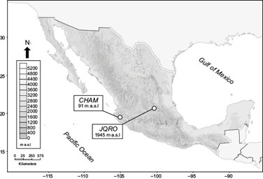
Fig. 1
Relief map depicting the orography of Mexico and the geographical location of the RUOA observatories chosen as sampling locations for this study.
Relief map depicting the orography of Mexico and the geographical location of the RUOA observatories chosen as sampling locations for this study.
2.2. Instrumentation
Each sampling site is equipped with sensors for measuring weather parameters (wind speed and direction, temperature, atmospheric pressure, solar radiation). It also features a TR-525M tipping-bucket rain gauge manufactured by Texas Electronics (www.texaselectronics.com) and an optical present weather sensor (PWS100) for precipitation assessment. The rain gauge has a resolution of 0.1 mm and an accuracy of 1% for rainfall rates up to 50 mm h−1. Water amounts are evaluated by the number of bucket overturns registered per minute, each one equivalent to 0.1 L m−2. Data from the TR-525M were used to select the sampling periods for this study, which were required to have a precipitation intensity greater than 10 mm h−1.
The PWS100 is a laser-based sensor consisting of a transmitter, four horizontal light sheets with a 0.4 mm spacing between them and a depth of 0.4 mm each, and two detectors. The laser’s wavelength is 830 nm. The instrument measures scattered light through an angle of 20º off the vertical and horizontal planes of the beam propagation axis to calculate the size and velocity of individual precipitation particles (Ellis et al., 2006) with an accuracy of 5% for both parameters and 10 % for total rain. The instrumental range for MOR estimates is up to 20 000 m with an accuracy of 10% for up to 10 000 m (Campbell Scientific, 2015). According to the manufacturer, the instrument configuration defines an area of 40 cm2 by the overlap of the measurement regions of the two detectors. The nominal detection sizes and fall velocities of individual particles range from 0.1 to 30 mm and from 0.1 to 30 m s−1, respectively. The outputs are arranged in 34 by 34 size and velocity bins. The device can distinguish between different classes of hydrometeors and delivers output messages indicating the type of particles detected, such as rain, snow, hail, and others.
-
Ellis et al., 2006New laser technology to determine present weather parametersMeasurement Science and Technology, 2006
-
Campbell Scientific, 2015PWS100 Present Weather Sensor. Instruction manual. Revision 9/15, 2015
The PWS100 geometry for visibility estimation is like that of other conventional sensors. By its design, the light forward scattered by atmospheric particles is used to estimate the atmosphere’s extinction coefficient. So, MOR estimation is based on the assumption that the absorption effect is not significant and that the light intensity collected by the detectors is proportional to the extinction coefficient (Ellis et al., 2006; Campbell Scientific, 2015).
-
Ellis et al., 2006New laser technology to determine present weather parametersMeasurement Science and Technology, 2006
-
Campbell Scientific, 2015PWS100 Present Weather Sensor. Instruction manual. Revision 9/15, 2015
The nominal range for particle diameter, D, was between 0.45 and 6 mm in this study. The upper value was established to avoid the influence of mixed rain (graupel and hail melting), as noted by Martínez and Gori (1999), and because field observations have few drops with D > 6 mm (Barros et al., 2010). On the other hand, the PWS100 algorithm excludes precipitation particles with anomalous velocities. Hydrometeor velocity is gathered when it crosses through the four light sheets. If the instrument detects a hydrometeor falling too fast for its size, it is categorized as an unknown particle and excluded from calculations. However, an additional particle with the same characteristics as the average of good particles falling at that time is included (Campbell Scientific, 2015). This process, in turn, leads to low counts of raindrops smaller than 0.4 mm given the occurrence of super-terminal drops in this size range (Montero-Martínez et al., 2009; Montero-Martínez and García-García, 2016). Furthermore, Agnew (2013), Johannsen et al. (2020), and Pickering et al. (2021) reported that the PWS100 underestimates the number of raindrops with D values < 0.8 mm. Thus, these instruments are suitable for rainfall events with significant liquid precipitation (Jia et al., 2020) when the number or proportion of large drops is dominant. Therefore, this study’s data analysis focused on precipitation events with periods of heavy (10.0 ≤ R < 50 mm h−1) and extremely heavy rainfall intensities (R ≥ 50 mm h−1) (WMO, 2018). The time resolution used for all instruments is 1 min, and the total number of samples available for this study was 4737.
-
Martínez and Gori (1999)Raindrop size distributions in convective clouds over CubaAtmospheric Research, 1999
-
Barros et al., 2010Size distribution of raindropsNature Physics, 2010
-
Campbell Scientific, 2015PWS100 Present Weather Sensor. Instruction manual. Revision 9/15, 2015
-
Montero-Martínez et al., 2009Do all raindrops fall at terminal speed?Geophysical Research Letters, 2009
-
Montero-Martínez and García-García, 2016On the behaviour of raindrop fall speed due to windQuarterly Journal of the Royal Meteorological Society, 2016
-
Agnew (2013)Final report on the operation of a Campbell Scientific PWS100 Present Weather Sensor at Chilbolton observatory, 2013
-
Johannsen et al. (2020)Comparison of three types of laser optical disdrometers under natural rainfall conditionsHydrological Sciences Journal, 2020
-
Pickering et al. (2021)Evaluation of multiple precipitation sensor designs for precipitation rate and depth, drop size and velocity distribution, and precipitation typeJournal of Hydrometeorology, 2021
-
Jia et al., 2020A comparison of precipitation measurements with a PWS100 laser sensor and a Geonor T-200B precipitation gauge at a Nival glacial zone in eastern Tianshan, Central AsiaAtmosphere, 2020
3. Material and methods
3.1. Methods
3.1.1. MOR (visibility) computations
The Beer-Lambert-Bouguer law empirically links the attenuation of energy with the properties of the substance it passes through. Using Koschmieder’s law (1924), an empirical relationship was obtained between the contrast (C) and the coefficient extinction that describes the optical properties of the air:
-
Koschmieder’s law (1924)Theorie der horizontalen sichweiteBeiträge zur Physik der Atmosphäre, 1924
e1C = B h - B 0 B h = B h - B h ( 1 - e - σ x ) B h = e - σ x
In this equation, B 0 and B h represent the apparent luminance of the black object and the horizon sky, respectively; σ (in m-1) is the light extinction coefficient, and x (in m) is related to a distance length. The World Meteorological Organization recommends a contrast threshold (ϵ) of 0.05 for purposes such as airport visibility (Horvath, 1981). Eq. (1) helps define the MOR (expressed in m or km). This parameter represents the path length in the atmosphere required to reduce the luminous flux in a collimated beam from an incandescent lamp at a color temperature of 2700 K to 5% of its original value (WMO, 2018).
-
Horvath, 1981Atmospheric visibilityAtmospheric Environment, 1981
-
WMO, 2018Guide to Instruments and Methods of Observation, 2018
e2M O R = 1 σ l n 1 ϵ = 1 σ l n 1 0.05 ≈ 3 σ
Eq. (2) establishes that MOR, as with visibility, is determined by the extinction coefficient of the air. Previous studies (Ulbrich and Atlas, 1985; Vasseur and Gibbins, 1996; Uijlenhoet et al., 2011) mention that σ can be theoretically evaluated from the DSD for rain events, in addition to via extinction efficiency (Q ext ), which is defined as the ratio of the extinction cross-section of raindrops (in mm2) to the geometric cross-section of the hydrometeors (in m2). In meteorological studies, DSD indicates the number of drops in a determined diameter range contained in a unit air volume, N(D), which is the number concentration (in m-3 mm-1). During a rain event, the DSD changes according to the number and size of the precipitating raindrops. Light rain is generally dominated by small and medium-sized drops (narrow DSD). However, when rainfall intensity increases, the number of large raindrops typically increases (broad DSD). The median volume diameter (D 0 , in mm) is used in radar meteorology to characterize the DSD broadness. D 0 is the upper raindrop diameter in the DSD that contributes to half of the total liquid water content (LWC) (Testud et al., 2001; Wen et al., 2016):
-
Ulbrich and Atlas, 1985Extinction of visible and infrared radiation in rain: Comparison of theory and experimentJournal of Atmospheric and Oceanic Technology, 1985
-
Vasseur and Gibbins, 1996Prediction of apparent extinction for optical transmission through rainApplied Optics, 1996
-
Uijlenhoet et al., 2011Path-average rainfall estimation from optical extinction measurements using a large-aperture scintillometerJournal of Hydrometeorology, 2011
-
Testud et al., 2001The concept of “normalized” distribution to describe raindrop spectra: A tool for cloud physics and cloud remote sensingJournal of Applied Meteorology and Climatology, 2001
-
Wen et al., 2016Statistical characteristics of raindrop size distributions observed in East China during the Asian summer monsoon season using 2-D video disdrometer and micro rain radar dataJournal of Geophysical Research: Atmospheres, 2016
e3∫ 0 D 0 D 3 N D d D = 1 2 ∫ 0 ∞ D 3 N D d D
Mie’s theory enables us to estimate the extinction cross-section of rain particles by assuming that raindrops have quasi-spherical shapes and their size, related to the equivalent spherical drop diameter (D, in mm), greatly exceeds the visible and near infra-red wavelengths. For raindrop sizes D > 0.2 mm, Q ext becomes 2 (Hansen and Travis, 1974; Gultepe et al., 2006), independent of the employed wavelength (Chýlek, 1977). Therefore, σ (in km-1) is related to the second moment of N(D) (Uijlenhoet et al., 2011):
-
Hansen and Travis, 1974Light scattering in planetary atmospheresSpace Science Reviews, 1974
-
Gultepe et al., 2006A new visibility parameterization for warm-fog applications in numerical weather prediction modelsJournal of Applied Meteorology and Climatology, 2006
-
Chýlek, 1977A note on extinction and scattering efficienciesJournal of Applied Meteorology and Climatology, 1977
-
Uijlenhoet et al., 2011Path-average rainfall estimation from optical extinction measurements using a large-aperture scintillometerJournal of Hydrometeorology, 2011
e4σ = π 2 × 10 - 3 ∫ 0 ∞ D 2 × N D d D
The PWS100 can calculate visibility values based on the type of particles detected in its sampling volume. When a DSD is obtained during a weather event, the instrument uses these data to provide better, accurate MOR estimates (Campbell Scientific, 2015).
-
Campbell Scientific, 2015PWS100 Present Weather Sensor. Instruction manual. Revision 9/15, 2015
The rainfall rate is calculated using the third moment of the DSD as:
e5R = 6 π × 10 - 4 ∫ 0 ∞ D 3 × v D × N D d D
Here, v (D) (in m s-1) is the mean fall speed of the raindrops detected in each size bin during sampling. Eqs. (4) and (5) indicate that DSD characteristics are crucial for describing visibility features and rain events. σ has been expressed as a function of R using power-law expressions (σ = aR b ) (Ulbrich and Atlas, 1985). Atlas (1953) noted that the coefficients of such equations are related to the DSD and associated the differences between the theoretical and empirical estimates of the coefficients in the σ-R relationships with the shape of the DSD. It should be noted that the a-coefficient of the expression can decrease by up to an order of magnitude as DSD broadens. Further, Ulbrich and Atlas (1985) and Uijlenhoet et al. (2011) settled that the exponent values in the σ-R expression are related to variations in the shape coefficients of the gamma distribution. Moreover, Shipley et al. (1974) and Miers (1983) reported that the coefficients also vary depending on the type of rainfall; namely, the exponent corresponding to thunderstorm cases is significantly larger than that for orographic ones (Uijlenhoet et al., 2011). Rahman et al. (2008) presented data of visibility < 1 km during periods of extreme rainfall (R > 100 mm h−1), and Gultepe and Milbrandt (2010) reported relationships between visibility and R for light, moderate, and heavy rainfalls.
-
Ulbrich and Atlas, 1985Extinction of visible and infrared radiation in rain: Comparison of theory and experimentJournal of Atmospheric and Oceanic Technology, 1985
-
Atlas (1953)Optical extinction by rainfallJournal of the Atmospheric Sciences, 1953
-
Ulbrich and Atlas (1985)Extinction of visible and infrared radiation in rain: Comparison of theory and experimentJournal of Atmospheric and Oceanic Technology, 1985
-
Uijlenhoet et al. (2011)Path-average rainfall estimation from optical extinction measurements using a large-aperture scintillometerJournal of Hydrometeorology, 2011
-
Shipley et al. (1974)Measurements of rainfall rates by lidarJournal of Applied Meteorology and Climatology, 1974
-
Miers (1983)Review of calculations of extinction for visible and infrared wavelengths in rain. (No. ERADCOM/ASL-TR-0134), 1983
-
Uijlenhoet et al., 2011Path-average rainfall estimation from optical extinction measurements using a large-aperture scintillometerJournal of Hydrometeorology, 2011
-
Rahman et al. (2008)Study of rain attenuation consequence in free space optic transmission, 2008
-
Gultepe and Milbrandt (2010)Probabilistic parameterizations of visibility using observations of rain precipitation rate, relative humidity, and visibilityJournal of Applied Meteorology and Climatology, 2010
3.2. Statistical analysis
Considering the differences in their operational principles, the PWS100 has advantages over the TR-525M for assessing the actual duration of precipitation events. An issue with tipping bucket rain gauges is that measurements are discreet, corresponding to fixed volumes of water that accumulate in a small bucket, resulting in a record of times that rainfall accumulation equals the bucket’s volume (Michaelides et al., 2009). When a rain episode is light, the bucket takes a long time to fill, and a desynchronization occurs insofar as it compares with an optical disdrometer. On the other hand, heavy rainfall yields rapid filling and emptying of the bucket, leading to water loss during the accumulation process. Rainwater estimates were evaluated using statistical metrics, specifically the Nash-Sutcliffe efficiency (NSE), the root mean square error (RMSE), and the percent bias (PBIAS).
-
Michaelides et al., 2009Precipitation: Measurement, remote sensing, climatology and modelingAtmospheric Research, 2009
The NSE is a dimensionless statistic that indicates how well the measured and reference data fit the 1:1 line. It ranges between −∞ and 1.0, with the latter value being the optimal (Nash and Sutcliffe, 1970). Based on this statistic, the performance evaluation will be non-acceptable when NSE < 0.5, satisfactory when 0.5 ≤ NSE < 0.6, good when 0.6 ≤ NSE < 0.8, and excellent when NSE ≥ 0.8 (Moriasi et al., 2015). RMSE is measured in units of accumulated rainwater (Acc, in mm) and represents the size of the typical difference between the measurements of the PWS100 and the TR-525M. It is usually accepted that a lower RMSE implies better model performance. Another criterion for interpreting the RMSE results is based on a report by Singh et al. (2005) in which RMSE is considered low when the result is less than half the standard deviation of the gauge estimates. Finally, PBIAS measures the average tendency of the observations, expressed as a percentage, as larger or smaller than reference measurements. The optimal value of PBIAS is 0.0, for which low-magnitude values suggest rainwater estimates that are very similar between the disdrometer and the rain gauge. The PBIAS parameter is interpreted (Walther and Moore, 2005) as an under- or over-estimation (corresponding to positive or negative values) concerning the reference value, i.e., the rain gauge. Based on the evaluation criteria given by Moriasi et al. (2015), the comparison between the instruments should be considered as not satisfactory when PBIAS > |0.25|.
-
Nash and Sutcliffe, 1970River flow forecasting through conceptual models. Part 1: A discussion of principlesJournal of Hydrology, 1970
-
Moriasi et al., 2015Hydrologic and water quality models: performance measures and evaluation criteriaTransactions of ASABE, 2015
-
Singh et al. (2005)Hydrologic modeling of the Iroquois River watershed using HSPF and SWATJournal of the American Water Resources Association, 2005
-
Walther and Moore, 2005The concepts of bias, precision and accuracy, and their use in testing the performance of species richness estimators, with a literature review of estimator performanceEcography, 2005
-
Moriasi et al. (2015)Hydrologic and water quality models: performance measures and evaluation criteriaTransactions of ASABE, 2015
Interpretation of the results is essential in extracting meaning from data and measurements. The effect size quantifies the difference between (two) groups. It has the advantage of emphasizing the size of the difference over the simple use of statistical significance tests (Coe, 2002; Sullivan and Feinn, 2012). This parameter is a major tool for interpreting the effectiveness of a particular phenomenon, providing relevant interpretation, and can be expressed as the Hedges effect size statistic g as shown below:
-
Coe, 2002It’s the effect size, stupid. What effect size is and why it is importantBritish Educational Research Association Annual Conference 12-14, September 2002, 2002
-
Sullivan and Feinn, 2012Using effect size-Or why the p value is not enoughJournal of Graduate Medical Education, 2012
e6g = X - 1 - X - 2 S
where X̅ 1 and X̅ 2 correspond to the mean values of the two groups to be compared, and S is the pooled sample standard deviation of the compared groups (Morales-Vallejo, 2008; Montero-Martínez and García-García, 2016; Goulet-Pelletier and Cousineau, 2018; Montero-Martínez, 2021). Cohen (1988) proposed guidelines for interpreting this magnitude (g): (1) 0.2 considered “small” (a real effect, indicating something is happening and can only be noticed through a careful study); (2) 0.5 considered “medium” (large enough to be visible to the naked eye); and (3) 0.8 considered “large” (which indicates absolute perceptible, i.e., a very substantial effect).
-
Morales-Vallejo, 2008Estadística aplicada a las ciencias sociales, 2008
-
Montero-Martínez and García-García, 2016On the behaviour of raindrop fall speed due to windQuarterly Journal of the Royal Meteorological Society, 2016
-
Goulet-Pelletier and Cousineau, 2018A review of effect sizes and their confidence intervals. Part I: The Cohen’s d familyThe Quantitative Methods for Psychology, 2018
-
Montero-Martínez, 2021The effect of altitude on the prediction of momentum for rainfall erosivity studies in MexicoCatena, 2021
-
Cohen (1988)Statistical power analysis for the behavioral sciences, 1988
The adjustment curve coefficients of the MOR-R and σ-R relationships were obtained with the Matlab software using the Levenberg-Marquardt (LM) algorithm and the nonlinear least-squares adjustment method. LM is an iterative technique that locates the minimum value of a function expressed as the sum of squares of nonlinear functions, and it applies to a wide variety of nonlinear least squares. The LM interpolation is based on the maximum neighborhood in which the truncated Taylor approximations adequately represent the nonlinear model. Each LM iteration determines its parameter step from the product of a damped inverse curvature matrix with a parameter space gradient (Levenberg, 1944; Marquardt, 1963; Lampton, 1997).
-
Levenberg, 1944A method for the solution of certain non-linear problems in least squaresQuarterly of Applied Mathematics, 1944
-
Marquardt, 1963An algorithm for the least-squares estimation of nonlinear parametersJournal of the Society for Industrial and Applied Mathematics, 1963
-
Lampton, 1997Damping-undamping strategies for the Levenberg- Marquardt nonlinear least-squares methodComputers in Physics, 1997
4. Results
4.1 Rainfall amounts
The performance of disdrometers and rain gauges at each sampling site was evaluated by comparing the measurements of accumulated rainwater per event. The sampling time is crucial for striking a balance between observing fluctuations and the inhomogeneity of the actual physical processes of rainfall. The data analysis in this study was based on 4373 observations of 1-minute rainfall periods corresponding to 16 rainy episodes, which showed periods of at least 5 min with rainfall intensities greater than 10 mm h−1 (i.e., heavy rain). Furthermore, a sub-selection of 676 periods that showed at least 100 drops detected with nominal sizes between 0.4 and 6.0 mm was used. As previously mentioned, this size diameter range was selected due to instrumental issues and to avoid the impact of mixed rain (Montero-Martínez et al., 2021).
-
Montero-Martínez et al., 2021Study of rain classification and the tendency of gamma DSD parameterizations in MexicoAtmospheric Research, 2021
Table I shows the results providing a descriptive analysis (mean and standard deviation) of the estimates of Acc per event detected by the TR-525M and the PWS100. The table also includes the NSE, PBIAS, and RMSE values as obtained for each sampling site. The average rainwater outcomes suggest that optical instruments gave greater estimates than the tipping-bucket rain gauge (TR-525M) for the specific dataset and agree with previous studies (Montero-Martínez and García-García, 2016; Liu et al., 2019; Montero-Martínez et al., 2020; Ro et al., 2024).
-
Montero-Martínez and García-García, 2016On the behaviour of raindrop fall speed due to windQuarterly Journal of the Royal Meteorological Society, 2016
-
Liu et al., 2019Comparative measurement of rainfall with a precipitation micro-physical characteristics sensor, a 2D video disdrometer, an OTT Parsivel disdrometer, and a rain gaugeAtmospheric Research, 2019
-
Montero-Martínez et al., 2020The change of rainfall kinetic energy content with altitudeJournal of Hydrology, 2020
-
Ro et al., 2024Comparative study of rainfall measurement by optical disdrometer, tipping-bucket rain gauge, and weighing precipitation gaugeNatural Hazards, 2024
Table I
Average and standard deviations (in parenthesis) of rainwater amount estimates for PWS100 and TR-525M data collected in each sampling site. Performance measures (NSE, PBIAS, and RMSE) were also obtained, considering the rain gauge as the reference.
Average and standard deviations (in parenthesis) of rainwater amount estimates for PWS100 and TR-525M data collected in each sampling site. Performance measures (NSE, PBIAS, and RMSE) were also obtained, considering the rain gauge as the reference.
| n e | Mean (SD) | NSE | PBIAS (%) | RMSE (mm) | ||
| PWS100 | TR-525M | |||||
| (mm) | (mm) | |||||
| CHAM | 9 | 23.7 (16.2) | 24.1 (19.7) | 0.9 | 1.9 | 4.3 |
| JQRO | 7 | 28.9 (18.2) | 25.4 (15.2) | 0.9 | 14.1 | 5.1 |
NSE was used to determine the relative magnitude of the residual variance between the PWS100 and TR-525M observations and the measured disdrometer variance (Nash and Sutcliffe, 1970). The results indicate the extent to which the disdrometer data correspond to the 1:1 line of a plot with the gauge estimates (Moriasi et al., 2015). The NSE results in Table I indicate very good performance levels for both instruments at both sampling sites (Moriasi et al., 2007). The RMSE values, being less than half the SD of the PWS100 observations, are considered low according to the criterion of Singh et al. (2005). PBIAS absolute values range from 2 to 14% using rainfall water accumulation estimates from the rain gauge as a reference. When comparing the performance evaluation statistic values for the JQRO site with those for CHAM, the values for the JQRO site are larger. However, the results presented in Table I indicate a good performance for both instruments in estimating the amount of rainfall in the sampling sites.
-
Nash and Sutcliffe, 1970River flow forecasting through conceptual models. Part 1: A discussion of principlesJournal of Hydrology, 1970
-
Moriasi et al., 2015Hydrologic and water quality models: performance measures and evaluation criteriaTransactions of ASABE, 2015
-
Moriasi et al., 2007Model evaluation guidelines for systematic quantification of accuracy in watershed simulationsTransactions of ASABE, 2007
-
Singh et al. (2005)Hydrologic modeling of the Iroquois River watershed using HSPF and SWATJournal of the American Water Resources Association, 2005
4.2 Behavior of the estimates of MOR
Figure 2 displays MOR data (gray lines) obtained from the PWS100, and rainfall intensity estimates gathered from the TR-525M over six rain episodes at the sampling sites. The analysis of the MOR scores in Figure 2 shows that the lowest values for this parameter (MOR < 1 km) are linked to the periods of highest R outcomes (R > 60 mm h−1), which not only agrees with the expectations but also with other reports. The disdrometer data indicate that the rain events lasted a minimum of three hours and illustrate the effect of this phenomenon (precipitation) on atmospheric visibility as associated with MOR data. The estimated maximum rainfall intensity for the events shown corresponds to periods of heavy and extreme precipitation (R > 10 mm h−1) lasting a few minutes. Ma et al. (2018) reported that a larger R in precipitation (or LWC in fog) led to an increase in the value of the extinction coefficient. Another factor that could contribute to the decrease in MOR estimates is the density of small droplets produced by the raindrops splashing on the ground. These droplets could be suspended for a few moments and then form a small layer of fog just above the surface. However, due to the specific conditions of the periods studied (high rainfall intensity with a temperature usually greater than 15 ºC), the appearance of fog is not observed. Therefore, the study of this factor is deemed implausible and falls outside the scope of the present study.
-
Ma et al. (2018)The scattering effects on the visibility measurements of laser transmissometer in rain and fogOptik, 2018
Thumbnail
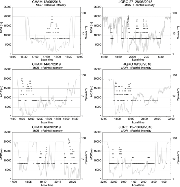
Fig. 2
Estimates of meteorological optical range (MOR, grey lines) and rainfall intensity collected during six rainfall events in two sites in Mexico. The temporal resolution is 1 min.
Estimates of meteorological optical range (MOR, grey lines) and rainfall intensity collected during six rainfall events in two sites in Mexico. The temporal resolution is 1 min.
4.3 Relationship between rainfall intensity and MOR
Figure 3 shows the MOR variations associated with the R estimates obtained from the TR-525M with R ≥ 12 mm h−1 for each sampling period. The estimates of MOR based on the extinction coefficient, gathered from DSD, as a function of R data from the PWS100 are also shown in grey symbols. The numbers of data points shown in the plots are 305 for CHAM and 371 for JQRO. The MOR data illustrate the expected behavior for periods with higher R values, during which an increase in the concentration of large raindrops produced more significant interactions with light and caused a MOR reduction in those episodes. Also, the MOR outcomes obtained directly from the optical disdrometer are observed to match those from the DSD data. The variability in the MOR data could be attributed to natural DSD fluctuations (Ulbrich and Atlas, 1985) that depend on environmental thermodynamic conditions (Gultepe and Milbrandt, 2010), such as relative humidity, atmospheric pressure, or temperature.
-
Ulbrich and Atlas, 1985Extinction of visible and infrared radiation in rain: Comparison of theory and experimentJournal of Atmospheric and Oceanic Technology, 1985
-
Gultepe and Milbrandt, 2010Probabilistic parameterizations of visibility using observations of rain precipitation rate, relative humidity, and visibilityJournal of Applied Meteorology and Climatology, 2010
Thumbnail
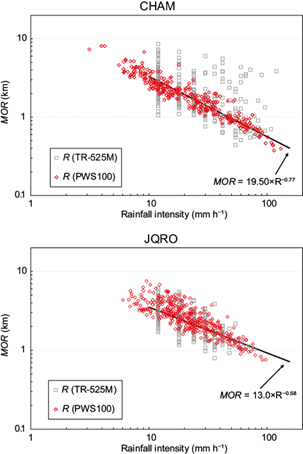
Fig. 3
Plots of meteorological optical range (MOR) data (km−1) from PWS100 versus rainfall intensity (R > 10 mm h−1) estimates with the rain gauge at 1-min rain intervals gathered at each site. The diagrams also display the MOR estimates using the extinction coefficient from raindrop size distribution (DSD) outcomes (open red diamonds). Each point corresponds to a sampling period during which at least 100 raindrops were detected by the PWS100.
Plots of meteorological optical range (MOR) data (km−1) from PWS100 versus rainfall intensity (R > 10 mm h−1) estimates with the rain gauge at 1-min rain intervals gathered at each site. The diagrams also display the MOR estimates using the extinction coefficient from raindrop size distribution (DSD) outcomes (open red diamonds). Each point corresponds to a sampling period during which at least 100 raindrops were detected by the PWS100.
Furthermore, Figure 3 also displays a power law MOR-R parameterization. It can be noticed that the power-law equation reasonably models the values of MOR when the precipitation is extreme (R > 50 mm h−1). Table II presents the performance evaluation of the fitting equations derived from the data collected at the sampling platforms used in this study. Based on the evaluation criteria provided by Moriasi et al. (2015), the coefficient of determination values in Table II (r2 > 0.95) indicate that the performance of the power-law model obtained for each site is very good. The RMSE results show a similar performance between the fitting equations obtained for each sampling site. However, the NSE criteria suggest that the performance of the models should be considered unsatisfactory because the obtained values are less than 0.45 (Moriasi et al., 2015).
-
Moriasi et al. (2015)Hydrologic and water quality models: performance measures and evaluation criteriaTransactions of ASABE, 2015
-
Moriasi et al., 2015Hydrologic and water quality models: performance measures and evaluation criteriaTransactions of ASABE, 2015
Table II
Performance measures for the MOR-R fitting expressions for each sampling site shown in Fig. 3.
Performance measures for the MOR-R fitting expressions for each sampling site shown in Fig. 3.
| n | MOR = aR b | |||
| r2 | RMSE (km) | NSE | ||
| CHAM | 305 | 0.99 | 1.29 | 0.16 |
| JQRO | 371 | 0.99 | 0.79 | 0.39 |
4.4 Relationship between the extinction coefficient and rainfall intensity
Figure 4 illustrates the σ estimates computed with the second DSD moment as a function of the rainfall rates calculated using the rain gauge measurements. Each panel displays a σ-R fit equation obtained for each sampling site, along with the corresponding coefficient of determination. The lines correspond to the expressions obtained with heavy precipitation data (R > 10 mm h−1).
Thumbnail
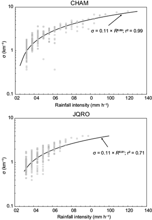
Fig. 4
Relationships of σ vs. R for heavy rainfall sampling periods at the selected measurement platforms. Continuous lines correspond to the results of the fitting equations (see details in the text).
Relationships of σ vs. R for heavy rainfall sampling periods at the selected measurement platforms. Continuous lines correspond to the results of the fitting equations (see details in the text).
Table III presents the fitting equations for the σ-R data shown in Figure 4. Data with R > 10 mm h−1 were used for the heavy rain adjustment (n represents the number of periods that met this requirement). The coefficients of the equations are expressed as the 95% confidence interval (CI). The a- and b-coefficients for the σ-R relationships are similar to those obtained by Shipley et al. (1974) using tipping bucket rain gauges to estimate the rainfall rates in thunderstorms and stratus rainfall. The effect size results suggest that the adjusted equation for JQRO differs slightly from the reference values, expressed as σ = (0.16 ± 0.04)R (0.74±0.12) . In the case of the equation obtained for CHAM, there is no significant difference between the coefficient and exponent outcomes with the reference values (probably because of the greater range of the intervals).
-
Shipley et al. (1974)Measurements of rainfall rates by lidarJournal of Applied Meteorology and Climatology, 1974
Table III
Results for the 95% confidence intervals from the coefficients of the fitting relationships between σ (in km−1) and R (in mm h−1) estimates and the corresponding performance measures of NSE and RMSE. Also, the Hedges’ effect size (g) outcomes are shown for the σ-R fitting equations as concerning to that reported by Shipley et al. (1974).
Results for the 95% confidence intervals from the coefficients of the fitting relationships between σ (in km−1) and R (in mm h−1) estimates and the corresponding performance measures of NSE and RMSE. Also, the Hedges’ effect size (g) outcomes are shown for the σ-R fitting equations as concerning to that reported by Shipley et al. (1974).
| n | Equation | g | NSE | RMSE (km−1) | ||
| a | b | |||||
| CHAM | 305 | σ = (0.11 ± 0.01)R (0.88±0.004) | 2.7 | 3.8 | 0.86 | 0.50 |
| JQRO | 371 | σ = (0.12±0.02)R(0.81±0.05) | 0.2 | 0.1 | 0.71 | 0.34 |
-
Shipley et al. (1974)Measurements of rainfall rates by lidarJournal of Applied Meteorology and Climatology, 1974
The exponent values of both expressions are consistent with those reported by Atlas (1953) and Miers (1983) and have implications for understanding precipitation events at the sampling sites. According to these authors, the σ-R power-law coefficients for Bergeron precipitation range from 0.15 to 0.38, whereas the exponents lie between 0.55 and 0.70. Moreover, the reported values for the a-coefficient are between 0.25 and 0.32 and close to 0.36 for widespread rain and thunderstorms, respectively. When orographic rain occurs, the a-coefficient changes by an order of magnitude, being between 1.25 and 2.6 (Atlas, 1953). The a-coefficient results in Figure 3 imply that the precipitation events studied here were caused by non-orographic rain. Furthermore, the b-exponent values obtained for both sampling sites are also consistent with those reported by Shipley et al. (1974) for rainfall from stratus and thunderstorm clouds (mixed clouds) and are significantly greater than those for orographic, warm rain (Atlas, 1953).
-
Atlas (1953)Optical extinction by rainfallJournal of the Atmospheric Sciences, 1953
-
Miers (1983)Review of calculations of extinction for visible and infrared wavelengths in rain. (No. ERADCOM/ASL-TR-0134), 1983
-
Atlas, 1953Optical extinction by rainfallJournal of the Atmospheric Sciences, 1953
-
Shipley et al. (1974)Measurements of rainfall rates by lidarJournal of Applied Meteorology and Climatology, 1974
-
Atlas, 1953Optical extinction by rainfallJournal of the Atmospheric Sciences, 1953
Based on Moriasi et al. (2015), the NSE outcomes obtained for the σ-R relationships indicate good (0.6 < NSE < 0.8) and very good (NSE > 0.8) performances for the JQRO and CHAM cases, respectively. Thus, these findings suggest that fitted parameterizations for heavy rain can also be used to estimate the extinction coefficient for periods with extreme rainfall.
-
Moriasi et al. (2015)Hydrologic and water quality models: performance measures and evaluation criteriaTransactions of ASABE, 2015
4.5 Variation of the extinction coefficient
The presence of large drops contributes a greater volume of water to the rain rate than smaller drops (Pickering et al., 2021). Willis (1984) and Willis and Tattelman (1989) reported that precipitation from warm-based convective clouds, such as those found at the sampling sites of this study, can be described using a gamma-distribution function. Montero-Martínez et al. (2021) demonstrated that all three gamma parameters decrease as R increases at the selected sampling locations, a finding that aligns with results from other studies conducted at diverse locations (Tokay and Short, 1996; Atlas and Ulbrich, 2006; Caracciolo et al., 2006). Figure 5 presents the R and D 0 (in mm) estimates for the rainy periods selected at the sampling sites. D 0 is used as a proxy of the DSD width. Atlas (1953) and Ulbrich (1983) demonstrated the relationship between D 0 and the DSD gamma distribution’s shape and slope parameters.
-
Pickering et al., 2021Evaluation of multiple precipitation sensor designs for precipitation rate and depth, drop size and velocity distribution, and precipitation typeJournal of Hydrometeorology, 2021
-
Willis (1984)Functional fits to some observed drop size distributions and parameterization of rainJournal of the Atmospheric Sciences, 1984
-
Willis and Tattelman (1989)Drop-size distributions associated with intense rainfallJournal of Applied Meteorology and Climatology, 1989
-
Montero-Martínez et al. (2021)Study of rain classification and the tendency of gamma DSD parameterizations in MexicoAtmospheric Research, 2021
-
Tokay and Short, 1996Evidence from tropical raindrop spectra of the origin of rain from stratiform versus convectiveJournal of Applied Meteorology, 1996
-
Atlas and Ulbrich, 2006Drop size spectra and integral remote sensing parameters in the transition from convective to stratiform rainGeophysical Research Letters, 2006
-
Caracciolo et al., 2006Analysis of the moments and parameters of a gamma DSD to infer precipitation properties: a convective stratiform discrimination algorithmAtmospheric Research, 2006
-
Atlas (1953)Optical extinction by rainfallJournal of the Atmospheric Sciences, 1953
Thumbnail
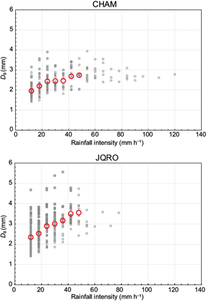
Fig. 5
Plots of D 0 outcomes calculated from disdrometer vs. rain gauge R estimates for the Chamela (CHAM) and Juriquilla (JQRO) sampling platforms. Red circles indicate the statistically significant D 0 averages for the rain gauge R categories. (D 0 : median volume diameter; R: rainfall rate.)
Plots of D 0 outcomes calculated from disdrometer vs. rain gauge R estimates for the Chamela (CHAM) and Juriquilla (JQRO) sampling platforms. Red circles indicate the statistically significant D 0 averages for the rain gauge R categories. (D 0 : median volume diameter; R: rainfall rate.)
The plots in Figure 5 show that the DSD broadens (as inferred by the increase in D 0 ) as R increases. Data dispersion is significant at the sampling sites. It is not straightforward to distinguish differences in the estimates between locations; however, the greater D 0 averages in JQRO with respect to CHAM suggest different rain producing microphysical processes. Moreover, the results show a similar tendency for maximum D 0 values when R > 50 mm h−1.
According to Ulbrich and Atlas (1985), the behavior of the σ-R parameters is opposite to each other: a decreases as b increases. The same authors also mention that the exponent on R is also related to the gamma shape parameter of the DSD gamma distribution parameterization: b increases as µ increases. Atlas (1953) asserted that the minimal exponent increments in power-law equations are due to the velocity change with drop size. Considering these statements and the outcomes in Figure 5, the values of the exponent in Table III are consistent. It is worth noting that the PWS100 underestimates the number of raindrops smaller than 0.8 mm, which results in overestimations of D 0 . Therefore, the exponent on R should have a value smaller than those reported in Table III.
-
Ulbrich and Atlas (1985)Extinction of visible and infrared radiation in rain: Comparison of theory and experimentJournal of Atmospheric and Oceanic Technology, 1985
-
Atlas (1953)Optical extinction by rainfallJournal of the Atmospheric Sciences, 1953
Considering the variations of σ with the width of the raindrop spectrum (characterized by D 0 or the DSD gamma distribution expression), our results point that the association between MOR and DSD is not a simple one and also depends on environmental (particulate matter concentrations) and thermodynamical (pressure, relative humidity, and others) factors in the sampling regions as noted by Gultepe and Milbrandt (2010).
-
Gultepe and Milbrandt (2010)Probabilistic parameterizations of visibility using observations of rain precipitation rate, relative humidity, and visibilityJournal of Applied Meteorology and Climatology, 2010
5. Summary and conclusions
Concurrent MOR values and microphysical measurements were collected at two sites in Mexico with different climatic and geomorphological characteristics to study the evolution of the former parameter during rain events. One sampling location is close to the Pacific Ocean coast (equatorial monsoon climate), whereas the other is in an urban area on the High Plateau of Mexico (cold semi-arid climate). Optical disdrometers (PWS100) were deployed in the sampling locations to gather data for these parameters from June 2018 to September 2019. Weather observations were obtained from meteorological stations installed on the same platforms.
The selected precipitation events have periods of rain with intensities greater than 10 mm h−1; therefore, this study focused on analyzing MOR changes during heavy and extreme rainfall. Estimates of total rainfall per event from PWS100 and rain gauges reveal an optical device overestimate (up to 15% based on the PBIAS outcomes) relative to the gauges due to the former’s better detection of light rain. Nevertheless, the NSE and RMSE results suggest that the performance of the instruments used to estimate precipitation at both study sites is satisfactory.
MOR and rainfall data in Figure 2 show that the most significant decreases in MOR scores are associated with heavy and extreme rainfall intensity periods. The MOR estimates derived from the extinction coefficient, evaluated using DSD outcomes from PWS100, are comparable to those collected directly from the instrument based on the forward scatter light.
A power-law type equation (σ = aR b ) was obtained for each event to fit the behavior of both parameters using the second DSD moment to estimate the extinction coefficient σ and tipping bucket rain gauge observations to compute rainfall intensity. The resulting coefficient values of the σ-R power-law fitted equations for the data sets collected in the selected sites (which were expressed as 95% CIs) are consistent with those obtained in previous studies for rainfall from mixed clouds (Bergeron type) or convective thunderstorms (Atlas, 1953; Miers, 1983; Uijlenhoet et al., 2011). However, the size effect outcomes revealed that differences concerning the reported values in Shipley et al. (1974) could be considered large for the case at CHAM. This underscores the need for further studies to establish a general σ-R relationship. The a-coefficient values are much closer to those related to thunderstorms or widespread rain than to others types, such as orographic rainfall (which are an order of magnitude higher). Furthermore, our b-exponent values in the σ-R fitted expressions are near those shown in Shipley et al. (1974), Miers (1983), and Uijlenhoet et al. (2011) for mixed-phase (thunderstorms) or non-orographic storms. Given that the reports regarding the PWS100 underestimate the number of small raindrops (D < 0.8 mm), which may generate an overestimation of D 0 , our values for the exponent on R would be slightly lower. Nonetheless, the NSE and RMSE values indicate adequate performance for the fitting equations at each sampling site.
-
Atlas, 1953Optical extinction by rainfallJournal of the Atmospheric Sciences, 1953
-
Miers, 1983Review of calculations of extinction for visible and infrared wavelengths in rain. (No. ERADCOM/ASL-TR-0134), 1983
-
Uijlenhoet et al., 2011Path-average rainfall estimation from optical extinction measurements using a large-aperture scintillometerJournal of Hydrometeorology, 2011
-
Shipley et al. (1974)Measurements of rainfall rates by lidarJournal of Applied Meteorology and Climatology, 1974
-
Shipley et al. (1974)Measurements of rainfall rates by lidarJournal of Applied Meteorology and Climatology, 1974
-
Miers (1983)Review of calculations of extinction for visible and infrared wavelengths in rain. (No. ERADCOM/ASL-TR-0134), 1983
-
Uijlenhoet et al. (2011)Path-average rainfall estimation from optical extinction measurements using a large-aperture scintillometerJournal of Hydrometeorology, 2011
For the locations and sampling periods of this study, visibility variation is a function of raindrop concentration. Our findings indicate that MOR (visibility) and extinction coefficient estimates during precipitation events at the sampling sites chosen for this study are closely related to rainfall intensity, specifically the large raindrop proliferation. Bulk parameters (rainfall intensity) can then be used to estimate MOR. However, the need for further studies to reduce the uncertainties of the expressions relating visibility to rain parameters is evident, especially during intense rainfall episodes when σ estimations do not adequately reflect the increased concentration of large raindrops. An alternative explanation would be to consider the cross-section variations due to the oscillations of these raindrops. The instruments used in this study do not provide any data on this phenomenon, so we could not explore the topic. Understanding these issues would enable us to better comprehend the interactions between electromagnetic radiation and hydrometeors and, in turn, improve transportation safety regarding visibility degradation. These results also suggest that practical application-fitted parameterizations for heavy rain can be used to estimate the extinction coefficient for periods with extreme rainfall, which could have significant implications in the fields of meteorology and hydrology, as well as in enhancing transport safety in Mexico.
Acknowledgments
The Red Universitaria de Observatorios Atmosféricos (RUOA) of the Universidad Nacional Autónoma de México provided the data used in this study. We thank staff members of RUOA María Eugenia González del Castillo, Delibes Flores Román and Omar Alejandro López Antón. This work was supported in part by the UNAM-DGAPA-PAPIIT (IN101921) program.
References
- Agnew J. 2013. Final report on the operation of a Campbell Scientific PWS100 Present Weather Sensor at Chilbolton observatory. Space RAL. Rutherford Appleton Laboratory Space, Science and Technology Facility Council, Swindon, UK. Links
- Atlas D. 1953. Optical extinction by rainfall. Journal of the Atmospheric Sciences 10: 486-489. https://doi.org/10.1175/1520-0469(1953)010<0486:OEBR>2.0.CO;2 Links
- Atlas D. 1964. Advances in radar meteorology. Advances in Geophysics 10: 317-478. https://doi.org/10.1016/S0065-2687(08)60009-6 Links
- Atlas D, Ulbrich C. 2006. Drop size spectra and integral remote sensing parameters in the transition from convective to stratiform rain. Geophysical Research Letters 33: L16803, https://doi.org/10.1029/2006GL026824 Links
- Barros AP, Prat OP, Testik FY. 2010. Size distribution of raindrops. Nature Physics 6: 232. https://doi.org/10.1038/nphys1646 Links
- Brodie I, Rosewell C. 2007. Theoretical relationships between rainfall intensity and kinetic energy variants associated with stormwater particle washoff. Journal of Hydrology 340: 40-47. https://doi.org/10.1016/j.jhydrol.2007.03.019 Links
- Campbell Scientific. 2015. PWS100 Present Weather Sensor. Instruction manual. Revision 9/15. Logan, Utah, Campbell Scientific. Available at: Available at: https://s.campbellsci.com/documents/us/manuals/pws100.pdf (accessed 2025 February 14) Links
- Caracciolo C, Prodi F, Battaglia A, Porcu F. 2006. Analysis of the moments and parameters of a gamma DSD to infer precipitation properties: a convective stratiform discrimination algorithm. Atmospheric Research 80: 165-186. https://doi.org/10.1016/j.atmosres.2005.07.003 Links
- Chen P, Wang P, Li Z, Yang Y, Jia Y, Yang M, Peng J, Li H. 2023. Raindrop size distribution characteristics of heavy precipitation events based on a PWS100 disdrometer in the Alpine mountains, eastern Tianshan, China. Remote Sensing 15: 5068. https://doi.org/10.3390/rs15205068 Links
- Chýlek P. 1977. A note on extinction and scattering efficiencies. Journal of Applied Meteorology and Climatology 16: 321-322. https://doi.org/10.1175/1520-0450(1977)016<0321:ANOEAS>2.0.CO;2 Links
- Coe R. 2002. It’s the effect size, stupid. What effect size is and why it is important. In: British Educational Research Association Annual Conference 12-14, September 2002. University of Exeter, Exeter, UK. Available at: Available at: https://f.hubspotusercontent30.net/hubfs/5191137/attachments/ebe/ESguide.pdf (accessed 2025 February 15) Links
- Cohen J. 1988. Statistical power analysis for the behavioral sciences. Lawrence Earlbaum Associates, Hillsdale, NJ. Links
- CNA. 2007. Normales climatológicas provisionales 1971-2000. Unidad del Servicio Meteorológico Nacional, Comisión Nacional del Agua, Mexico City. Available at: Available at: https://smn.conagua.gob.mx/es/climatologia/informacion-climatologica/normales-climatologicas-por-estado?estado=jal (accessed 2025 February 14) Links
- Díaz-Infante S, Lara C, Arizmendi MC. 2020. Temporal dynamics of the hummingbird-plant interaction network of a dry forest in Chamela, Mexico: A 30-year follow-up after two hurricanes. PeerJ 8:e8338. Available at: Available at: https://peerj.com/articles/8338/ (accessed 2025 February 14) Links
- Dunlop S. 2008. A dictionary of weather. 2nd ed. Oxford University Press [online]. https://doi.org/10.1093/acref/9780199541447.001.0001 Links
- Duthon P, Colomb M, Bernardin F. 2019. Light transmission in fog: The influence of wavelength on the extinction coefficient. Applied Sciences 9: 2843. https://doi.org/10.3390/app9142843 Links
- Eidels-Dubovoi S. 2002. Aerosol impacts on visible light extinction in the atmosphere of Mexico City. Science of The Total Environment 287: 213-220. https://doi.org/10.1016/s0048-9697(01)00983-4 Links
- Ellis RA, Sandford AP, Jones GE, Richards J, Petzing J, Coupland JM. 2006. New laser technology to determine present weather parameters. Measurement Science and Technology 17: 1715-1722. https://doi.org/10.1088/0957-0233/17/7/009 Links
- EPA. 1979. Protecting Visibility. An EPA report to Congress. EPA/450-5-79-008. U.S. Environmental Protection Agency, Research Triangle Park, NC. Available at: Available at: https://nepis.epa.gov/Exe/ZyPDF.cgi?Dockey=P1003OJ9.pdf (accessed 2025 February 14) Links
- Gires A, Tchiguirinskaia I, Schertzer D. 2018. Two months of disdrometer data in the Paris area. Earth System Science Data 10: 941-950. https://doi.org/10.5194/essd-10-941-2018 Links
- Goulet-Pelletier JC, Cousineau D. 2018. A review of effect sizes and their confidence intervals. Part I: The Cohen’s d family. The Quantitative Methods for Psychology 14: 242-265. https://doi.org/10.20982/tqmp.14.4.p242 Links
- Gultepe I, Müller MD, Boybeyi Z. 2006. A new visibility parameterization for warm-fog applications in numerical weather prediction models. Journal of Applied Meteorology and Climatology 45: 1469-1480. http://www.jstor.org/stable/26171867 Links
- Gultepe I, Milbrandt JA. 2010. Probabilistic parameterizations of visibility using observations of rain precipitation rate, relative humidity, and visibility. Journal of Applied Meteorology and Climatology 49: 36-49. https://doi.org/10.1175/2009JAMC1927.1 Links
- Gultepe I, Sharman R, Williams PD, Zhou B, Ellrod G, Minnis P, Trier S, Griffin S, Yum SS, Gharabaghi B, Feltz W, Temimi M, Pu Z, Storer LN, Kneringer P, Weston MJ, Chuang Hy, Thobois L, Dimri AP, Dietz SJ, França GB, Almeida MV, Neto FLA. 2019. A review of high impact weather for aviation meteorology. Pure and Applied Geophysics 176: 1869-1921. https://doi.org/10.1007/s00024-019-02168-6 Links
- Hansen JE, Travis LD. 1974. Light scattering in planetary atmospheres. Space Science Reviews 16: 527-610. https://doi.org/10.1007/BF00168069 Links
- Horvath H. 1981. Atmospheric visibility. Atmospheric Environment 15: 1785-1796. https://doi.org/10.1016/0004-6981(81)90214-6 Links
- ICAO. 2005. Manual of runway visual range observing and reporting practices. Doc 9328 AN/908. International Civil Aviation Organization, Montreal. Available at: Available at: https://amc.namem.gov.mn/wp-content/uploads/2022/Documents/icao/19.pdf?_t=1638837870 (accessed 2025 February 17) Links
- Huang J, Cao Y, Raimundo X, Cheema A, Salous S. 2019. Rain statistics investigation and rain attenuation modeling for millimeter wave short-range fixed links. IEEE Access 7: 156110-156120. https://doi.org/10.1109/access.2019.2949437 Links
- Jia Y, Li Z, Xu C, Jin S, Deng H. 2020. A comparison of precipitation measurements with a PWS100 laser sensor and a Geonor T-200B precipitation gauge at a Nival glacial zone in eastern Tianshan, Central Asia. Atmosphere 11: 1079. https://doi.org/10.3390/atmos11101079 Links
- Johannsen LL, Zambon N, Strauss P, Dostal T, Neumann M, Zumr D, Cochrane TA, Blöschl G, Klik A. 2020. Comparison of three types of laser optical disdrometers under natural rainfall conditions. Hydrological Sciences Journal 65: 524-535. https://doi.org/10.1080/02626667.2019.1709641 Links
- Koschmieder H. 1924. Theorie der horizontalen sichweite. Beiträge zur Physik der Atmosphäre 12: 171-181. Links
- Kottek M, Grieser J, Beck C, Rudolf B, Rubel F. 2006. World map of the Köppen-Geiger climate classification updated. Meteorologische Zeitschrift 15: 259-263. https://doi.org/10.1127/0941-2948/2006/0130 Links
- Lampton M. 1997. Damping-undamping strategies for the Levenberg- Marquardt nonlinear least-squares method. Computers in Physics 11: 110-115. https://doi.org/10.1063/1.168600 Links
- Lee J, Chae J, Yoon T, Yang H. 2018. Traffic accident severity analysis with rain-related factors using structural equation modeling-A case study of Seoul City. Accident Analysis and Prevention 112: 1-10. https://doi.org/10.1016/j.aap.2017.12.013 Links
- Levenberg K. 1944. A method for the solution of certain non-linear problems in least squares. Quarterly of Applied Mathematics 2: 164-168. https://doi.org/10.1090/qam/10666 Links
- Liaw JJ, Lian SB, Huang YF, Chen RC. 2009. Atmospheric visibility monitoring using digital image analysis techniques. In: Computer analysis of images and patterns (Jiang X, Petkov N, Eds.). Springer, Berlin. https://doi.org/10.1007/978-3-642-03767-2_146 Links
- Liu X, He B, Zhao S, Hu S, Liu L. 2019. Comparative measurement of rainfall with a precipitation micro-physical characteristics sensor, a 2D video disdrometer, an OTT Parsivel disdrometer, and a rain gauge. Atmospheric Research 229: 100-114. https://doi.org/10.1016/j.atmosres.2019.06.020 Links
- Liu Z, Chen Y, Gu X, Yeoh JKW, Zhang Q. 2022. Visibility classification and influencing-factors analysis of airport: A deep learning approach. Atmospheric Environment 278: 119085. https://doi.org/10.1016/j.atmosenv.2022.119085 Links
- Ma Y, Liu W, Gao H, Chen N, Xiong X. 2018. The scattering effects on the visibility measurements of laser transmissometer in rain and fog. Optik 157: 957-967. https://doi.org/10.1016/j.ijleo.2017.11.150 Links
- Marquardt DW. 1963. An algorithm for the least-squares estimation of nonlinear parameters. Journal of the Society for Industrial and Applied Mathematics 11: 431-441. https://doi.org/10.1137/0111030 Links
- Martínez D, Gori EG. 1999. Raindrop size distributions in convective clouds over Cuba. Atmospheric Research 52: 221-239. https://doi.org/10.1016/S0169-8095(99)00020-4 Links
- Michaelides S, Levizzani V, Anagnostou E, Bauer P, Kasparis T, Lane JE. 2009. Precipitation: Measurement, remote sensing, climatology and modeling. Atmospheric Research 94: 512-533. https://doi.org/10.1016/j.atmosres.2009.08.017 Links
- Middleton WEK. 1957. Vision through the atmosphere. In: Geophysik II/Geophysics II. Handbuch der Physik/Encyclopedia of physics, vol. 10/48. Springer-Verlag, Berlin. https://doi.org/10.1007/978-3-642-45881-1_3 Links
- Miers BT. 1983. Review of calculations of extinction for visible and infrared wavelengths in rain. (No. ERADCOM/ASL-TR-0134). Atmospheric Sciences Laboratory, US Army Electronics Research and Development Command, White Sands Missile Range, NM. Available at: Available at: https://apps.dtic.mil/sti/tr/pdf/ADA132659.pdf (accessed 2025 February 17) Links
- Montero-Martínez G, Kostinski AB, Shaw RA, García-García F. 2009. Do all raindrops fall at terminal speed? Geophysical Research Letters 36: L11818. https://doi.org/10.1029/2008GL037111 Links
- Montero-Martínez G, García-García F. 2016. On the behaviour of raindrop fall speed due to wind. Quarterly Journal of the Royal Meteorological Society 142: 2013-2020. https://doi.org/10.1002/qj.2794 Links
- Montero-Martínez G, García-García F, Arenal-Casas S. 2020. The change of rainfall kinetic energy content with altitude. Journal of Hydrology 584: 124685. https://doi.org/10.1016/j.jhydrol.2020.124685 Links
- Montero-Martínez G. 2021. The effect of altitude on the prediction of momentum for rainfall erosivity studies in Mexico. Catena 207: 105604. https://doi.org/10.1016/j.catena.2021.105604 Links
- Montero-Martínez G, Gómez-Balvás SS, García-García F. 2021. Study of rain classification and the tendency of gamma DSD parameterizations in Mexico. Atmospheric Research 252: 105431. https://doi.org/10.1016/j.atmosres.2020.105431 Links
- Morales-Vallejo P. 2008. Estadística aplicada a las ciencias sociales. Universidad Pontificia Comillas, Madrid, Spain. Links
- Moriasi DN, Arnold JG, van Liew MW, Bingner RL, Harmel RD, Veith TL. 2007. Model evaluation guidelines for systematic quantification of accuracy in watershed simulations. Transactions of ASABE 50: 885-900. https://doi.org/10.13031/2013.23153 Links
- Moriasi DN, Gitau MW, Pai N, Daggupati P. 2015. Hydrologic and water quality models: performance measures and evaluation criteria. Transactions of ASABE 58: 1763-1785. https://doi.org/10.13031/trans.58.10715 Links
- Nash JE, Sutcliffe JV. 1970. River flow forecasting through conceptual models. Part 1: A discussion of principles. Journal of Hydrology 10: 282-290. https://doi.org/10.1016/0022-1694(70)90255-6 Links
- Pickering BS, Neely RR, Jeffery J, Dufton D, Lukach M. 2021. Evaluation of multiple precipitation sensor designs for precipitation rate and depth, drop size and velocity distribution, and precipitation type. Journal of Hydrometeorology 22: 703-720. https://doi.org/10.1175/JHM-D-20-0094.1 Links
- Rahman AK, Anuar MS, Aljunid SA, Junita MN. 2008. Study of rain attenuation consequence in free space optic transmission. In: Proceedings of the IEEE 6th National Conference on Telecommunication Technologies and IEEE 2nd Malaysia Conference on Photonics, Putrajaya, Malaysia, 64-70. https://doi.org/10.1109/NCTT.2008.4814239 Links
- Ro Y, Chang KH, Hwang H, Kim M, Cha JW, Lee C. 2024. Comparative study of rainfall measurement by optical disdrometer, tipping-bucket rain gauge, and weighing precipitation gauge. Natural Hazards 120: 2829-2845. https://doi.org/10.1007/s11069-023-06308-z Links
- RUOA. 2023. Red Universitaria de Observatorios Atmosféricos [dataset]. Available at: Available at: https://www.ruoa.unam.mx/ (accessed 2025 February 17) Links
- Shipley ST, Eloranta EW, Weinman JA. 1974. Measurements of rainfall rates by lidar. Journal of Applied Meteorology and Climatology 13: 800-807. https://doi.org/10.1175/1520-0450(1974)013<0800:MORRBL>2.0.CO;2 Links
- Singh J, Knapp HV, Demissie M. 2005. Hydrologic modeling of the Iroquois River watershed using HSPF and SWAT. Journal of the American Water Resources Association 41: 343-360. https://doi.org/10.1111/j.1752-1688.2005.tb03740.x Links
- Sullivan GM, Feinn R. 2012. Using effect size-Or why the p value is not enough. Journal of Graduate Medical Education 4: 279-282. https://doi.org/10.4300/JGME-D-12-00156.1 Links
- Testud J, Oury S, Black RA, Amayenc P, Dou X. 2001. The concept of “normalized” distribution to describe raindrop spectra: A tool for cloud physics and cloud remote sensing. Journal of Applied Meteorology and Climatology 40: 1118-1140. https://doi.org/10.1175/1520-0450(2001)040%3C1118:TCONDT%3E2.0.CO;2 Links
- Tokay A, Short D. 1996. Evidence from tropical raindrop spectra of the origin of rain from stratiform versus convective. Journal of Applied Meteorology 35: 355-371. https://doi.org/10.1175/1520-0450(1996)035<0355:EFTRSO>2.0.CO;2 Links
- Torres DS, Porrà JM, Creutin J-D. 1994. A general formulation for raindrop size distribution. Journal of Applied Meteorology and Climatology 33: 1494-1502. https://doi.org/10.1175/1520-0450(1994)033<1494:AGFFRS>2.0.CO;2 Links
- Uijlenhoet R, Cohard J, Gosset M. 2011. Path-average rainfall estimation from optical extinction measurements using a large-aperture scintillometer. Journal of Hydrometeorology 12: 955-972. https://doi.org/10.1175/2011JHM1350.1 Links
- Ulbrich CW, Atlas D. 1985. Extinction of visible and infrared radiation in rain: Comparison of theory and experiment. Journal of Atmospheric and Oceanic Technology 2: 331-339. https://doi.org/10.1175/1520-0426(1985)002<0331:EOVAIR>2.0.CO;2 Links
- Vasseur H, Gibbins CJ. 1996. Prediction of apparent extinction for optical transmission through rain. Applied Optics 35: 7144-7150. https://doi.org/10.1364/AO.35.007144 Links
- Wang S, Chen T, Yu B, Sun Y, Qin X. 2021. Coupling impacts of spray and rainfall on road visibility and vehicle speeds: A simulation-based analysis. Canadian Journal of Civil Engineering 49: 1220-1230. https://doi.org/10.1139/cjce-2021-0402 Links
- Walther BA, Moore JL. 2005. The concepts of bias, precision and accuracy, and their use in testing the performance of species richness estimators, with a literature review of estimator performance. Ecography 28: 815-829. https://doi.org/10.1111/j.2005.0906-7590.04112.x Links
- Wen L, Zhao K, Zhang G, Xue M, Zhou B, Liu S, Chen X. 2016. Statistical characteristics of raindrop size distributions observed in East China during the Asian summer monsoon season using 2-D video disdrometer and micro rain radar data. Journal of Geophysical Research: Atmospheres 121: 2265-2282. https://doi.org/10.1002/2015JD024160 Links
- Willis PT. 1984. Functional fits to some observed drop size distributions and parameterization of rain. Journal of the Atmospheric Sciences 41: 1648-1661. https://doi.org/10.1175/1520-0469(1984)041%3C1648:FFTSOD%3E2.0.CO;2 Links
- Willis PT, Tattelman P. 1989. Drop-size distributions associated with intense rainfall. Journal of Applied Meteorology and Climatology 28: 3-15. https://doi.org/10.1175/1520-0450(1989)028<0003:DSDAWI>2.0.CO;2 Links
- WMO. 2014. Guide to meteorological observing and information distribution systems for aviation weather services. WMO-No. 731. World Meteorological Organization, Geneva. Available at: Available at: https://library.wmo.int/idurl/4/31903 (accessed 2025 February 17) Links
- WMO. 2018. Guide to Instruments and Methods of Observation. Vol. I: Measurements of meteorological variables. WMO-No. 8. World Meteorological Organization, Geneva. Available at: Available at: https://library.wmo.int/idurl/4/68695 (accessed 2025 February 17) Links
- Zahid O, Huang J, Salous S. 2020. Long term rain attenuation measurements at millimeter wave bands for direct and side short-range fixed links. XXXIIIrd General Assembly and Scientific Symposium of the International Union of Radio Science, Rome, Italy, 1-4. https://doi.org/10.23919/URSIGASS49373.2020.9232024 Links
- Zhang Z, Guo H, Kang H, Wang J, An J, Yu X, Lv J, Zhu B. 2022. A new method for calculating average visibility from the relationship between extinction coefficient and visibility. Atmospheric Measurement Techniques 15: 7259-7264. https://doi.org/10.5194/amt-15-7259-2022 Links
- Zhuang Z, Li J, Chan PW, Tai H. 2022. Substitutability research for forward-scatter meters in indoor low-visibility environments. Meteorological Applications 29: e2050. https://doi.org/10.1002/met.2050 Links