nueva página del texto (beta)
 Inglés (pdf)
 Artículo en XML
 Referencias del artículo
 Enviar artículo por email
 Citado por SciELO
  Similares en
SciELO
Similares en
SciELO 
 Permalink
1. Introduction
Solar radiation is the primary energy source for the systems that govern the dynamics of the biosphere (Ortiz-Solorio, 2015). In conjunction with other factors, such as water and nutrients, plants can complete their biological cycle under optimal temperature and soil quality (physical and chemical). The impact of these factors on plant growth and development has been analyzed by various research areas, including agronomic sciences, botany, and ecology. However, it is essential to observe and analyze the nature of each factor before considering their study as a whole.
The amount of energy received by the Earth in the exosphere layer is an average of 1353 J m-2 s (Ortiz-Solorio, 2015); however, approximately 50% of the total energy is received by the Earth’s surface due to atmospheric interference, of which 20% is reflected; clouds absorb 4%; water, dust particles, and O3 absorb 16%; and the remaining 10% is dispersed in the air (Ben-Othman et al., 2018). In turn, this energy exhibits fluctuations in time and space due to the position of the sun in relation to a geographic location, which is determined by solar geometry parameters including solar height, declination, and azimuth, as well as the solar obliquity angle and solar time (Méndez-Pérez and Gómez-Azpeitia, 2015). The fraction of the resulting energy is again reflected as a function of surface properties, a behavior known as albedo. It allows an understanding of each terrestrial element’s reflectance, energy absorption capacity, and environmental interaction (Wickham et al., 2015).
In agriculture, the study of solar radiation focuses on the transformation of energy into biomass through the process known as photosynthesis, mainly the length of photosynthetically active radiation (PAR) (400 to 700 nm) by interfering with leaf expansion, pigment formation, stomata elongation, and therefore, yield (Zárate-Martínez et al., 2021; Sandoval-Rangel et al., 2022). On the other hand, ultraviolet (UV) lengths A (320 to 400 nm) and B (280 to 320 nm) have presented effects on fruit quality (Quintero-Arias et al., 2021), yield (Lycoskoufis et al., 2022), and interfere in the production of active compounds (Duo et al., 2019) and germination (Foroughbackhack-Pournavab et al., 2019), among others.
Various methods have been used by agricultural technicians to interfere with light interception on leaves (Unigarro et al., 2021). Among these are the selection of population density (Mena-Lorenzo et al., 2018), selective pruning and production in greenhouse systems using plastics to generate better light distribution (Sandoval-Rangel et al., 2022), implementation of artificial lighting systems using fluorescent or LED lamps (Contreras-Avilés, 2020), and installation of mulches. Mulches provide several beneficial effects, such as weed and pest control, moisture, and nutrient retention (Montemayor-Trejo et al., 2018; Sanjuán-Martínez et al., 2022). Orozco-Santos et al. (2023) demonstrated a significant difference in plant biomass when establishing plots with mulches of different colors (white, aluminum, green, and black) compared to bare soil, concluding that the white cover provided the greatest amount of biomass.
Soria et al. (1998) refer to this behavior as the absorption capacity and distribution of energy reflected by each type of surface due to its physical properties and the effect of color, where white surfaces reflect more light (Sánchez and Moreno, 2017) so that the percentage of reflected radiation can be used by plants, favoring photosynthetic and photostimulant processes (Wang et al., 2021). It is essential to establish an analysis method and predictive models to understand the radiation reflectance capacity of different surfaces. These models will be fundamental for selecting materials that optimize plant biomass production.
Some authors, such as Boscaini et al. (2019) and Contreras-Sepúlveda et al. (2021), utilize predictive radiation models based on the formulas of Prescott (1940) and Almorox et al. (2005), primarily for ecological, agronomic, and photovoltaic applications. However, due to the complexity of the fundamental values, researchers have established models based on the relationship between radiation values and the climatic variables of a region (Obando et al., 2019), such as temperature (Camayo-Lapa et al., 2019), cloud cover (Zhou et al., 2024), and wind speed (Estela-Urbina et al., 2019), among others, since these elements have a highly significant relationship, presenting changes during the year.
Fluctuations in radiation and climatic variables are considered in monitoring and analysis techniques for planning various agricultural activities, particularly the establishment of planting and harvesting dates for crops, thus affecting their yield and quality. Estimated values are generated from data acquired by various radiation monitoring instruments, including remote sensing techniques, and essential meteorological variables provided by weather stations, which offer real-time information, enabling the analysis of changes in climatological factors and vegetation development over time (Zuluaga et al., 2021). However, access to the platforms is limited, in most cases, for residents of a locality, so they focus on using established estimation models or the use of easily obtained manual sensors, allowing for accurate data to be obtained by being sensitive to the presence of light. Based on the various predictions, it is possible to design and plan strategies for utilizing solar energy at the local level.
In recent decades, time series analysis has enabled the understanding of seasonal patterns and trends over time (Box et al., 2015). Predictive models for variables of interest organized in terms of time have been developed by authors such as Camayo-Lapa et al. (2019), which differ from traditional predictive models of simple or multiple regression, where variables do not require a temporal order. Likewise, Vesga-Ferreira et al. (2022) mention that, although prediction using known linear techniques can provide accurate data, they may generate greater imprecision because the values of interest over time present a non-constant mean and variance. In conjunction with other characteristics of the time series, various advanced autoregressive methods can be implemented to forecast radiation in a location by collecting and recording past data to predict future events, making it possible to use it in areas of the financial sector, electric utilities, and environment (Yang et al., 2017; Valderrama-Balaguera et al., 2021).
The sequence is analyzed based on the analysis objective and the observed data; in turn, some methods allow for the supplementation of missing data recorded in the sensors due to various technical or human errors (García-Acevedo et al., 2016). The Holt-Winters model, also known as the exponential smoothing model (Bowerman et al., 2007), is used for time series prediction by decomposing it into three components: level (L), trend (T), and seasonality (S). L represents the base value of the time series at a given point in time; T captures the direction and speed of change in the level, while S reflects the repetitive patterns that occur at regular intervals.
Based on analyses, the impact of recent or historically observed values on the predicted estimates can be determined compared to traditional predictive models, such as multiple linear regression. In the present study, a comparison of two types of regression analysis was performed: multiple linear regression and time series regression by the Holt-Winters method for the forecast of incident solar radiation and its reflectance on surfaces with anti-weed covers in two shades, and a surface without cover, for the production of plant biomass for agricultural purposes during one year.
2. Materials and methods
2.1 Study area
Solar radiation values were captured at the geographic coordinates 25º47’6.79” N and 100º 17’ 12.5” W at an altitude of 504 masl. The maximum and minimum temperatures in the area range between 29.5 and 17.3 ºC. The average annual precipitation is reported to be 422.8 mm (INEGI, 2024).
2.2 Solar radiation monitoring
The monitoring of global UV A and B radiation, incident photosynthetically active radiation (PAR), and their respective reflectance on various surfaces was recorded daily for one year, from August 2022 to July 2023. The recording of radiation during a day was made based on the solar angle 60º and -60º for solar height in a horizontal plane and 0º for the highest point of the sun (zenith), corresponding to 08:00, 12:00 and 16:00 solar or astronomical hours (Rehman and Halawani, 1997). In other words, radiation monitoring was conducted at three daily monitoring times over one year. Likewise, the monitoring time was adjusted using Duffie and Beckman’s (1991) equation of time (ET), allowing for the addition or subtraction of minutes to solar time due to differences in the Earth’s translational motion speed (Table I). On the other hand, Mexico has four time zones. In the northern zone, the study site is located in the central time zone; therefore, we used the time zone based on the 90º meridian to adjust the civil time (CT) formula of Méndez-Pérez and Gómez-Azpeitia (2015).
Table I Models for adjusting the rotation time of the Earth.
| Variable | Model | Where |
| Equation of time | ET = 9.87 sin 2ƒ - 7.53 cos ƒ - 1.5 sin ƒ | ƒ = 360 (- 81)/364 (in degrees) JD: Julian day |
| Civil time of Mexico | CT = TSV - ET - 4(L - L’) | TSV: true solar time; ET: equation of time; L: geographic reference longitude; L’: geographic longitude of the site |
2.3 Evaluated surfaces and manual sensors
The evaluated surfaces were covered with polypropylene anti-weed nets and classified into three categories: covered with white polypropylene anti-weed nets (WPN), covered with black polypropylene anti-weed nets (BPN), and soil without cover (SWC). They were established in divided plots of 9 m2 each (Fig. 1a) without shade interference from buildings or trees at any time of the day.
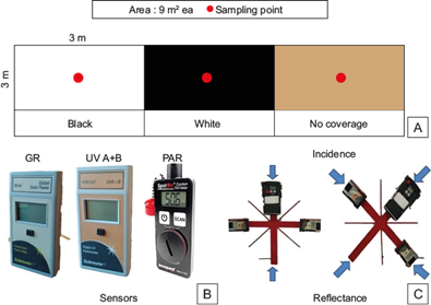
Fig. 1 (a) Evaluated surfaces covered with anti-weed netting and uncovered soil, (b) manual sensors, and (c) base for capturing incident and reflected radiation.
Daily solar radiation incidence and reflectance values were captured simultaneously with a portable solar meter sensor for global radiation (GR) (Solarmeter model 10.0), UV A + B radiation with a sensitive UV A + B meter (Solarmeter model 5.7), and photosynthetically active radiation (PAR) with a quantum meter (Spot0n Quantum PAR Light Meter 35650), with an accuracy of ± 80º from the vertical position of each sensor.
The sensors (Fig. 1b) were placed on a structure equipped with a set of fins that rotated around an axis, allowing the capture of solar radiation incidence and reflectance data at different tilt angles with respect to the zenith, as shown in Figure 1c. The rotating base was positioned 1 m above the surface, elevated from the lower end of the base, to collect the reflected radiation. On the other hand, the site’s climatic values (cloudiness, temperature, and relative humidity) were obtained at the same frequency as solar radiation monitoring using a hygrothermometer (Extech Instruments 445702) located at the study site facilities.
2.4 Descriptive analysis of incident solar radiation and statistical comparison of its reflectance.
Incident GR, UV A + B radiation, and PAR were analyzed over the year, identifying the maximum, minimum, and average values obtained at the sampling points. On the other hand, the reflectance of the evaluated surfaces was analyzed based on Jacobson’s albedo index (Jacobson, 1999). The indices are key to evaluating the balance of solar radiation on the surface and its impact on the environment, allowing for the determination of solar radiation energy use (Iturbide, 2020) and its application in various agricultural activities. Likewise, the amount of reflected radiation on the evaluated surfaces was compared using a Tukey test at a significance level of 95%.
2.5 Predictive models
Predictive models are a fundamental tool for understanding and predicting solar radiation over time at a specific site, which is crucial for informed decision-making in various agricultural activities. The ability to provide accurate estimates is a function of the precision and the amount of observed data, as well as the model that better fits the information obtained. There are several methods for analyzing and forecasting solar radiation. However, each model provides a different analytical perspective; therefore, two predictive models were employed in this research: the multiple regression model and the Holt-Winters model for time series analysis, as implemented in the R software (v. 3.6.0).
The analysis was performed using the sliding window method, which consists of analyzing a fixed-size section of data that is shifted along the time series. This method enables capturing the temporal evolution of a variable’s patterns in both training and test sets. The size of the sliding training window was 600 observations, and the test window consisted of 10 observations. The layout of the windows was visualized as follows: first training and test: X1, X2, X3,……X600 | X601,….X610; second training and test: X2, X3, X4,……X601 | X602,….X611.
Holt-Winters and multiple regression predictive models were performed on each sliding window and fitted to the previous observations for continuous analysis. Based on the above, a final model was obtained in each predictive method by fitting the individual models.
2.5.1 Multiple linear regression models
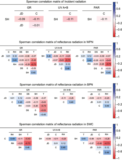
Multiple regression models were performed using the solar geometry parameters (Duffie and Beckman, 1991), the climate variables of the study site, and the monitoring times (Table II), which were significant in relation to the variables of incident solar radiation and its reflectance on the evaluated surfaces. The values were obtained simultaneously with the monitoring of solar radiation frequencies. The selection of independent variables was performed using the stepwise method, and the significant correlation between the independent variables was determined by the Spearman method at a significance level of p < 0.05.
Table II Independent variables analyzed for solar radiation estimation models.
| Solar geometry | Climate elements | Monitoring times | |
| Solar height (SH) | Sen h = senδ senφ + cosδ cosφω where: h: solar altitude in degrees δ: solar declination in degrees φ: site latitude in degrees ω: hour angle in degrees | Cloudiness (C%) | Julian day (JD) from 1 to 365 |
| Distance from the sun (DS) | (d m /DS)2 = 1 + 0.033 cos (2π/365 JD) where: d: distance from the Earth to the Sun in millions of km dm: mean distance: 149.6 million km JD: Julian day | Temperature ºC (T) | Civil time in decimals (CT) |
| Relative humidity (RH%) | |||
Subsequently, the dependent and independent variables were processed by standardizing the data to stabilize the variance before generating the models. Therefore, the abbreviations for solar height and earth to sun distance variables in the present investigation are indicated as SH and DS, respectively, to avoid confusion with the actual values obtained in the original formulas. The multiple regression model is expressed as follows:
where Y i is the response variable, β 0 is the constant value, β 1 ,…,β n are the regression coefficients, and X 1 ,…, X n are the independent variables.
2.5.2 Time series
The GR, UV A + B, and PAR radiation values analyses performed during the year were distributed in a time series. The locally estimated scatterplot smoothing (LOESS) method was applied to the time series to develop a local smoothing curve, which visualizes the trends in the observed data over the course of the year. Then a test for changes in the half was performed using two methods: (a) the sctest function at a significance level of 95%, where p values < 0.05 indicate significant changes in radiation values over time. (Zeileis et al., 2002), and (b) the analytical formula of the segmented regression (y t ) based on the Bayesian information (BIC) and the sum of squares of residuals (RSS) widely used for model fitting by identifying the points of structural changes in the time series, so that it is possible to evaluate the variation of radiation over the year (Box et al., 2015)
where y t is the dependent variable at time t, x t is the independent variable at time t, β 0,1 and β 1,j are regression coefficients for segment j, ε t is the error term at time t, and Ƭ 1 is the i-th change point.
where k is the number of model parameters, In(L) is the likelihood function of the estimated model, and n is the number of observations in the data.
2.5.3 Holt-Winters models
The Holt-Winters models were made based on the values of a single variable corresponding to global radiation, UV A + B, incident photosynthetically active radiation, and its reflectance on the evaluated surfaces. The formula predicts future values, considering the time series L, T, and S components (Bowerman et al., 2007).
where Lt is the level component, Tt is the trend component, and St is the seasonality component. Here, t represents the current time period, k is the number of steps ahead for forecasting (i.e., the forecast horizon), and m denotes the duration of the seasonal cycle.
The exponential smoothing factors range from 0 to 1, indicating the impact of observed values over time on the estimated values obtained using the Holt-Winters formula. Indices close to 0 indicate a more significant impact on past observations, while indices close to 1 indicate a greater weight on recent observations (Hyndman and Athanasopoulos, 2018). The formulas for updating the components based on the smoothing factors correspond to:
where α is the smoothing parameter for the level (0 < α < 1), y t is the observed value at time t, and S t-m is the seasonal component of the same period in the previous cycle (m periods back).
where β is the smoothing parameter for trend (0 < β ≤ 1) and L t - L t-1 is the change in level between periods t and t-1
where γ is the smoothing parameter for seasonality (0 < γ < 1) and y t - L t is the part of the observed value not explained by the current level.
The Holt-Winters analysis was performed by decomposing the additive time series, given the limited amount of observed data (< 1 year), assuming the seasonal component to be constant. Likewise, through decomposition, it is possible to observe patterns and trend changes according to the moving average and identify fluctuations that the model cannot explain (Hyndman and Athanasopoulos, 2018). On the other hand, a test for changes in structure was performed at a significance level of p < 0.05 to identify excessive fluctuations that would influence the model fits (Zeileis et al., 2002).
2.5.4. Comparison of predictive models
The predictive models were evaluated based on the performance metrics obtained from the forecast, considering the coefficient of determination R2, the root mean square error (RMSE), the mean absolute error (MAE), and the mean absolute percentage error (MAPE), where:
where y t represents the observed values, ŷ i are the predicted values, Ȳ is the mean of the observed values, and T and n are the total number of observations.
Multiple metrics enable a more comprehensive evaluation of model performance by providing analysis from different perspectives. The values of R2 indicate the fit of the models, while RMSE, MAE, and MAPE help identify different types of error, aiding in choosing a model that provides more accurate and reliable predictions (Yajure, 2023).
3. Results
3.1. Descriptive radiation analysis
The values of GR, UV A + B radiation, and PAR) (Fig. 2) presented maximum values in June with 753.7 ± 298.7 Wm-2, 2.9 ± 1.6 m Wm-2, and 1273.3 ± 525.8 µmol, respectively, and minimum values reported in November with 318.7 ± 362.8 Wm-2, 1.2 ± 1.6 m Wm-2 and 626.57 ± 650.36 µmol, respectively, corresponding to the monitored wavelengths.
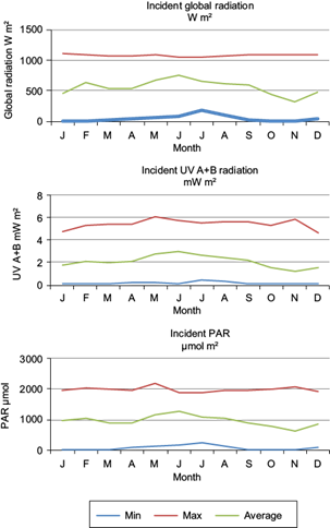
Fig. 2 Maximum, minimum, and average monthly values of GR, UV A + B, and incident PAR. (GR: global radiation; UV A + B: ultraviolet A and B radiation; PAR: photosynthetically active radiation.)
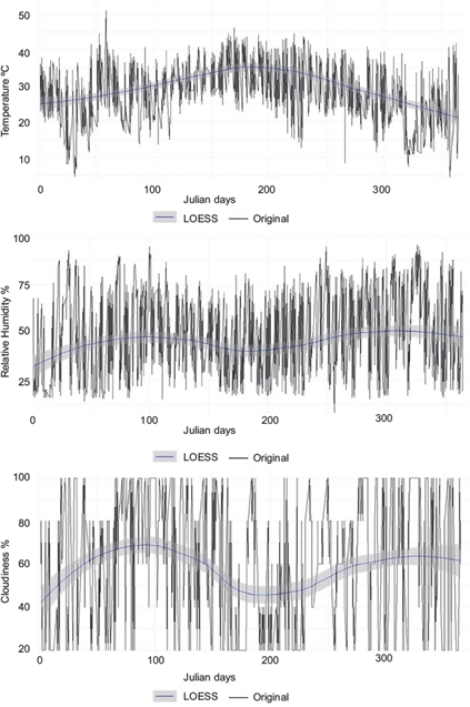
On the other hand, temperature ranges from 4.5 to 46 ºC and relative humidity from 8 to 96% were recorded (Fig. S1 in the supplementary material), registering an increase in the middle of the year when integrating the daily mean values. Relative humidity and cloudiness exhibited similar behavior, with their percentages decreasing as radiation and temperature values increased, and vice versa, as observed in the LOESS smoothing curve.
The reflected radiation on the WPN, BPN, and SWC surfaces exhibited a value of p < 0.05, so there is a statistically significant difference between half of the three surfaces corresponding to the different wavelengths evaluated, where the maximum values were in WPN with an annual average of 144.2 ± 110.1 Wm-2 of GR, 0.09 ± 0.1 m Wm-2 of UVA + B and 233.6 ± 181.4 µmol of PAR, followed by SWC with values of 79.4 ± 57.7 Wm-2, 0.01 ± 0.03 m Wm-2 and 70.7 ± 55.5 µmol, respectively. Meanwhile, BPN was observed at 36.8 ± 26.7 Wm-2, 0.05 ± 0.01 m Wm-2 and 54.1 ± 39.8 µmol, obtaining a higher absorbance percentage in the different wavelengths (Table III), reaching an albedo index of 0.14, similar to asphalt surfaces, concrete and urban areas according to Jacobson’s (1999) classification. The WPN obtained an index of 0.4, similar to that of old snow, while SWC registered 0.22 on average, similar to the classification ranges for soil.
Table III Reflectance values and average solar radiation percentage absorption on screened surfaces and uncovered soil.
| GR Wm-2 | UV A + B m Wm-2 | PAR µmol | |||||||
| Surfaces | |||||||||
| WPN | BPN | SWC | WPN | BPN | SWC | WPN | BPN | SWC | |
| Min | 3 | 0 | 2 | 0 | 0 | 0 | 6.4 | 0.5 | 2.3 |
| Max | 461 | 158 | 245 | 0.4 | 0.2 | 0.2 | 698 | 173 | 347.1 |
| Absorbance (%) | 60.6 | 90.9 | 78.4 | 96.3 | 96.8 | 99.6 | 64.5 | 92.9 | 81.3 |
GR: global radiation; UV A + B: ultraviolet A and B radiation; PAR: photosynthetically active radiation; WPR: white polypropylene anti-weed nets; BPN: black polypropylene anti-weed nets; SWC: soil without cover.
The sensors captured minimum values of zero in both GR and UV A + B on the different surfaces under completely cloudy sky conditions. This behavior can be attributed to the sensors’ sensitivity to radiation; the PAR sensor has a higher sensitivity capability, allowing it to capture radiation independently of weather conditions.
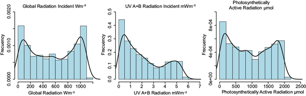
3.3. Normality tests
Normality tests of GR, UV A + B, and PAR incidence values, as well as their reflectance, presented a significance level of p < 0.05. Therefore, the observed values do not have a normal distribution. The normality histograms (Fig. 3) of GR and PAR show a bimodal distribution, indicating that the values present two more common values observed at the extremes of the histogram. In contrast, UV A + B presented a higher frequency in values close to zero. Based on the above, the observed values were standardized before the predictive models were performed.
3.4. Predictive models
The results of the stepwise method indicated that the independent variables of solar height (SH), Julian day (JD), and cloudiness (C) were significant for incident solar radiation (Fig. S2 in the supplementary material). On the other hand, in addition to the variables mentioned above, relative humidity (RH), distance from the Earth to the Sun (DS), and temperature (T) are included in the reflective solar radiation, whereas civil time (CT) was not found to be significant. However, Pearson’s correlation test indicated a high correlation (p > 0.7) between RH and T, so RH was excluded to avoid the multicollinearity effect in the prediction models, that is, the high correlation between two or more variables that would make difficult to estimate the values (Villegas-Guerrero et al., 2024).
3.4.1. Multiple regression models
The multiple regression models generated for the different lengths and movement of incident radiation (Fig. 4 and Table IV) and reflecting radiation (Table V) were obtained from the independent variables significant in relation to radiation, as well as from the model adjustments performed using the sliding window method. The final models obtained R2 values ranging from R2 > 0.50, providing an adequate fit due to the high relationship between the independent variables which presented a high correlation with the variable of interest, allowing accurate estimates to be obtained, except for UV A + B, which is reflected in SWC. It is worth mentioning that estimating incident radiation requires fewer independent variables compared to the radiation reflected on the different surfaces to obtain an adequate model fit (WPN, BPN, and SWC).
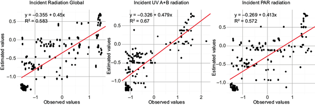
Fig. 4 Observed vs. predicted values of (a) global radiation, (b) UV A + B radiation, and (c) incident photosynthetically active radiation from the multiple regression models.
Table IV Multiple regression models of incident solar irradiance.
| Radiation | Model | R2 | |
| GR | = | -0.04 + 0.463 SH - 0.448 C - 0.061 JD | 0.58 |
| UV A + B | = | -0.051 + 0.692 SH - 0.284 C | 0.66 |
| PAR | = | -0.066 + 0.49 SH - 0.42 C | 0.57 |
GR: global radiation; UV A + B: ultraviolet A and B radiation; PAR: photosynthetically active radiation; SH: solar height; C: cloudiness; JD: Julian day.
Table V Multiple regression models of solar reflective radiation.
| Surface | Radiation | Model | R2 | |
| WPN | GR | = | -0.06 + 0.587 SH + 0.026 DS - 0.048 C + 0.503 T + 0.163 JD | 0.69 |
| UV A + B | = | -0.109 +0.63 SH - 0.125 C + 0.287 T + 0.239 JD | 0.49 | |
| PAR | = | -0.06 + 0.609 SH + 0.027 DS - 0.152 C - 0.356 T + 0.121 JD | 0.59 | |
| BPN | GR | = | -0.063 + 0.357 SH + 0.027 DS - 0.102 C + 0.525 T + 0.002 JD | 0.60 |
| UV A + B | = | -0.076 + 0.439 SH - 0.126 C - 0.186 RH | 0.37 | |
| PAR | = | -0.053 + 0.403 SH - 0.119 C - 0.395 RH - 0.077 JD | 0.36 | |
| SWC | GR | = | -0.034 + 0.58 SH - 0.148 N + 0.318 T | 0.66 |
| UV A + B | = | -0.044 + 0.392 SH - 0.088 C - 0.083 RH + 0.178 JD | 0.15 | |
| PAR | = | -0.081 + 0.505 SH - 0.286 C + 0.236 T + 0.005 JD | 0.52 | |
WPR: white polypropylene anti-weed nets; BPN: black polypropylene anti-weed nets; SWC: soil without cover; GR: global radiation; UV A + B: ultraviolet A and B radiation; PAR: photosynthetically active radiation; SH: solar height; C: cloudiness; T: temperature; RH: relative humidity; JD: Julian day.
The SH variable increases solar radiation, indicating that the levels of the dependent variable are a function of the sun’s position throughout the day and the year. On the other hand, temperature positively affects radiation, while the increase in the values of C and RH results in its decrease.
3.4.2 Time series
The time series of the GR, UV A + B, and PAR obtained a value of p < 0.05 with the sctest function, indicating that there are changes in the mean radiation over the year. In addition, using the Bayesian information criterion (BIC) it is observed that in the different wavelengths, there are two points of structural changes indicated in the BIC and SSR graphs (Fig. 5).
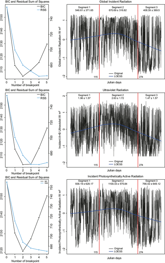
Fig. 5 Changes in the mean values of GR, UV A + B, and incident PAR presented in the time series and LOESS smoothing line. (GR: global radiation; UV A + B: ultraviolet A and B radiation; PAR: photosynthetically active radiation; LOESS: locally estimated scatterplot smoothing.)
The changes in the structure of the time series using the analítical formula of the segmented regression recorded trend changes in the values of the half radiation between 116 and 273 JD, dividing the time series into 3 segments. Likewise, the LOESS smoothing line allowed observing an asymmetric curve in segment 2, where a máximum value of the mean was obtained as shown in figure 6, followed by segment 1 from 1 to 115 JD, and the lowest values in segment 3 at the end of the year (274 to 365 JD), allowing a more precise analysis of the changes in radiation trends over the course of the year.
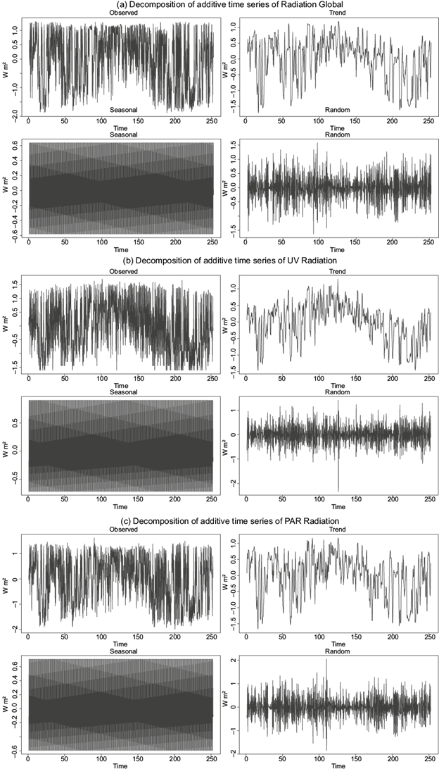
3.4.2. Holt-Winters models
The decomposition graphs of the solar radiation time series (Fig. 7) do not show a positive or negative trend defined in the behavior of radiation over the year; however, it is possible to witness a greater intensity of radiation in the middle of the year corresponding to the summer season, similar to the movement of the solar declination at an angle of 23.45º. On the other hand, the error graph shows that every 50 days, there are approximately eight to 11 repetitive erratic movements generated by factors that the model cannot explain.
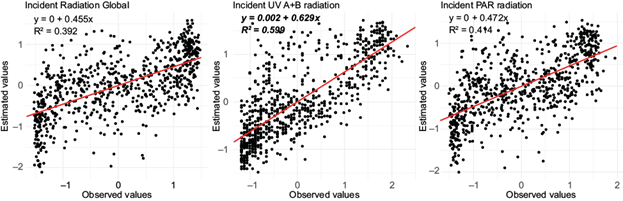
Fig. 7 Observed vs. predicted values of (a) GR, (b) UV A + B, and (C) incident PAR from the Holt-Winters models. (GR: global radiation; UV A + B: ultraviolet A and B radiation; PAR: photosynthetically active radiation.)
Tests for structural changes in the bands of agricultural interest showed a value of p > 0.05. Thus, it is established that values predicted by the Holt-Winters model do not exhibit significant changes, so the solar radiation analysis can be explained using a general model without requiring adjustments from multiple models.
The Holt-Winters models generated for the different lengths and movements of incident radiation (Fig. 7) and reflective radiation (Table VI) yielded a lower fit than the multiple regression models, with R2 values between 0.12 and 0.68. In other words, the temporal order can explain between 3 and 30% of radiation behavior over the year. It is pertinent to note that Holt-Winters models are generated solely with the variable of interest, i.e., univariate, thereby excluding the effect of environmental variables.
Table VI Holt-Winters models of incident and relativistic radiation.
| Flow | Surface | Radiation | Model | R2 | ||||
| L | T | S1 | S2 | S3 | ||||
| Incident | GL | -0.035 | -0.001 | -0.208 | 0.573 | -0.365 | 0.39 | |
| UV A + B | 0.374 | -0.036 | -0.358 | 0.993 | -0.634 | 0.55 | ||
| PAR | 0.174 | -2e-04 | -0.325 | 0.817 | -0.491 | 0.41 | ||
| Reflected | WPN | GL | -0.011 | -1e-04 | -0.186 | 0.668 | -0.482 | 0.68 |
| UV A + B | -0.346 | 6e-0.4 | -0.221 | 0.796 | -0.575 | 0.5 | ||
| PAR | -0.163 | -6e-04 | -0.163 | 0.722 | -0.558 | 0.63 | ||
| BPN | GL | -0.075 | 0.012 | -0.087 | 0.741 | -0.654 | 0.49 | |
| UV A + B | 0.098 | 2e-04 | -0.399 | 1.155 | -0.756 | 0.44 | ||
| PAR | 0.235 | -0.001 | -0.384 | 0.954 | -0.570 | 0.55 | ||
| SWC | GL | -0.201 | -3e-04 | -0.297 | 0.901 | -0.603 | 0.49 | |
| UV A + B | -0.250 | 9e-04 | -0.60 | 0.294 | -0.134 | 0.12 | ||
| PAR | 0.629 | -0.001 | -0.380 | 0.679 | -0.298 | 0.38 | ||
L: level component; T: trend component; S: seasonality component; GR: global radiation; UV A + B: ultraviolet A and B radiation; PAR: photosynthetically active radiation; WPR: white polypropylene anti-weed nets; BPN: black polypropylene anti-weed nets; SWC: soil without cover.
The general model of incident radiation indicates a positive effect of the L or level component on the observed values, while the trend (T) generates a negative behavior (Table VI). On the other hand, the values of L and T in the reflectance vary for GR and UV compared to PAR. S1, S2, and S3 represent the effect of seasonality according to the number of periods corresponding to the monitoring time per day. S2 values represented by the zenith will obtain positive values, both in the incident and reflected radiation flux, compared to S1 and S3 when obtaining negative values due to the lower amount of radiation received at sunrise and sunset times, respectively.
The exponential smoothing factors alpha, beta, and gamma control the L, T, and S components, respectively, of the Holt-Winters model. In Table VII, all three factors have indices close to 0, i.e., changes in the level, trend, and seasonality of solar radiation, UV A + B, and PAR will be a function of historically recorded or older values (Hyndman and Athanasopoulos, 2018).
Table VII Smoothing factors of the Holt-Winters model for time series.
| Flow | Surface | Radiation | Factors | ||
| α | β | γ | |||
| Incident | GR | 0.19 | 1e-04 | 0.05 | |
| UV A + B | 0.06 | 1e-04 | 0.05 | ||
| PAR | 0.13 | 1e-04 | 0.05 | ||
| Reflected | WPN | GR | 0.12 | 1e-04 | 0.07 |
| UV A + B | 0.04 | 1e-04 | 0.06 | ||
| PAR | 0.11 | 1e-04 | 0.03 | ||
| BPN | GR | 0.04 | 1e-04 | 0.07 | |
| UV A + B | 0.04 | 1e-04 | 0.09 | ||
| PAR | 0.16 | 1e-04 | 0.07 | ||
| SWC | GR | 0.10 | 1e-04 | 0.04 | |
| UV A + B | 0.006 | 1e-04 | 0.11 | ||
| PAR | 0.13 | 1e-04 | 0.09 | ||
GR: global radiation; UV A + B: ultraviolet A and B radiation; PAR: photosynthetically active radiation; WPR: white polypropylene anti-weed nets; BPN: black polypropylene anti-weed nets; SWC: soil without cover.
3.2.3. Model evaluation metrics
The performance of the models was evaluated using the RMSE, MAE, and MAPE metrics (Table VIII). The multiple regression model exhibited fewer large or outlier errors, achieving a lower RMSE than the Holt-Winters model while also yielding smaller errors, as indicated by the MAE. Nevertheless, the MAPE presented very high values in both models due to the transformation of the data.
Table VIII Evaluation metrics of the pre-productive solar radiation models.
| Flow | Surface | Radiation | Multiple regression | Holt-Winters | ||||
| RMSE | MAE | MAPE | RMSE | MAE | MAPE | |||
| Incident | GR | 0.70 | 0.52 | 174 | 0.78 | 0.63 | 225 | |
| UV A + B | 0.60 | 0.44 | 62 | 0.64 | 0.50 | 165 | ||
| PAR | 0.73 | 0.58 | 122 | 0.76 | 0.62 | 207 | ||
| Reflective | WPN | GR | 0.45 | 0.35 | 53 | 0.57 | 0.43 | 216 |
| UV A + B | 0.65 | 0.47 | 109 | 0.63 | 0.47 | 263 | ||
| PAR | 0.60 | 0.44 | 133 | 0.61 | 0.47 | 160 | ||
| BPN | GR | 0.51 | 0.36 | 70 | 0.74 | 0.54 | 257 | |
| UV A + B | 0.72 | 0.54 | 60 | 0.76 | 0.51 | 259 | ||
| PAR | 0.83 | 0.61 | 111 | 0.66 | 0.51 | 223 | ||
| SWC | GR | 0.44 | 0.35 | 100 | 0.63 | 0.50 | 225 | |
| UV A + B | 0.79 | 0.47 | 103 | 0.92 | 0.50 | 184 | ||
| PAR | 0.48 | 0.41 | 359 | 0.75 | 0.55 | 243 | ||
RMSE: root mean square error; MAE: mean absolute error; MAPE: mean absolute percentage error; GR: global radiation; UV A + B: ultraviolet A and B radiation; PAR: photosynthetically active radiation; WPR: white polypropylene anti-weed nets; BPN: black polypropylene anti-weed nets; SWC: soil without cover.
4. Discussion
Solar radiation is fundamental to atmospheric processes and crucial for life. Analyzing its behavior over time generates new challenges and opportunities to promote a more efficient and sustainable use of energy. In the present work, the amount of solar radiation in the lengths PAR and UV A + B reflected on surfaces covered with meshes used for weed control is analyzed to understand its fluctuations throughout the year from this perspective, which can be part of the decision-making process for using solar radiation resources in plants for agricultural purposes.
Over the last seven years, a significant increase in temperature and global radiation has been observed at the study site, compared to the data reported by Leal-Iga and Leal-Iga (2015), with differences of approximately 6 ºC and 0.45 kW h m-2, respectively. Barnes et al. (2019) note that changes in ozone layer thickness are a factor that has significantly influenced the increase in solar radiation, causing climatic changes such as temperature increases, and consequently affecting the responses of different crops (Medina-García et al., 2020). Therefore, it is recommended to redesign strategies for utilizing solar energy in future generations of crops without compromising their growth and yields.
Land surfaces present modifications according to the use granted, causing changes in the absorption and reflectance of solar radiation (Moreno-Arteaga et al., 2021); this behavior can be observed in CN, CB, and SC surfaces with an evident difference in the amount of reflected radiation (Table III), with maximum absorbance values in CN. High absorbance values can interfere with other processes in the soil due to the large amount of energy converted into heat that modifies soil conditions (Ben-Othman et al., 2018); likewise, changes in the amount of radiation will influence photosynthate and stomatal aperture (Hernández-Pérez et al., (2021) resulting in better plant development compared to production without the installation of the material (Montemayor-Trejo et al., 2018).
The balance of solar radiation on each evaluated surface can be measured using the surface or terrestrial albedo (Jacobson, 1999), a measurement index that allows evaluating the radiation received in a horizontal plane or with a certain angle of inclination, being relevant in the values of net solar radiation (Iturbide et al., 2020). The variation in the indices is a function of the properties of each surface, such as materials, presence of moisture, material thickness, porosity, roughness, and amount of vegetation present, among others, which has been supported in recent decades by Hernández and Montaner (2009) and confirmed by the review provided by Zhang et al. (2022). On the other hand, BPN and WPN mulches are made of polypropylene; hence, the color or hue determines the difference in albedo due to the ability of light surfaces to reflect more radiation compared to dark surfaces (Cheela et al., 2021), having a significant effect on the yield and quality of agricultural products (Escobosa-García et al., 2022). However, this also depends on the wavelength measured.
The analysis of incident UV radiation is associated with effects on the morphological, anatomical, and biochemical characteristics of plants (Badmus et al., 2022; Bernardo et al., 2024), and its absorption from surfaces may degrade installed plastics over time (Burrows et al., 2024). Meanwhile, PAR has been analyzed to assess the development and nutrient status of various crops (Minetti and Rivas, 2020; Sandoval-Rangel et al., 2022). The modification of these lengths generates significant changes (positive or negative) in plants; hence some authors, such as Cabral et al. (2020) and Peñaranda et al. (2020), proposed practices to improve their distribution and promote vegetative growth. The present research provides another perspective of analysis of the amount of absorbed and reflected radiation of UV A + B and PAR that can occur in anti-weed nets during the year (Table III), providing complementary information to demonstrate the efficiency in the installation of mulch types, such as those observed by Escobosa-García et al. (2022).
The analysis and estimation of solar radiation through various predictive models facilitate decision-making for its optimal use in the agricultural sector, considering climate factors due to the highly statistically significant relationship. The relationship between these variables is reflected in several studies, such as Ocampo and Rivas (2013), who found that temperature, relative humidity, and cloudiness were the most influential variables for radiation estimation, with a high correlation (R2 > 0.8) in most of the variables provided by weather stations.
On the other hand, Vélez-Pereira et al. (2015) compared the performance of simple and multivariate regressions, concluding that multiple regressions offered more apparent interpretations and ease of implementation, as well as a lower MAE margin when implementing the variables of temperature, humidity, and sunshine hours, similar to the highly correlated variables in the predictive multiple regression models obtained in the present study. Cloudiness and relative humidity in the model determine the values of solar radiation, i.e., in the presence of these two independent variables, a decrease in the dependent variable is estimated. Babar et al. (2019) referred to this behavior as the presence of various particles, such as water molecules, dispersed in the atmosphere, resulting in the scattering of light and, therefore, a decrease in solar radiation (Zhang et al., 2023).
Multiple regression models are considered pointwise, i.e., they do not require an order in time, making them a suitable tool for estimating solar radiation. However, their efficiency depends mainly on the selected independent variables and the accuracy of the observed values to achieve optimal model performance. However, the increase in radiation in recent years underscores the need for a more comprehensive analysis as a function of time.
The time series is a set of observations used to analyze the behavior of the variable of interest, to identify trends, points of changes in the mean, and errors in the course (Mejía-Vásquez and González-Chávez, 2019) as the random fluctuations observed in the decomposition of solar radiation (Fig. 6) due to the movement of the Earth around the Sun, which has been proven and described previously. Likewise, Arunkumar et al. (2021) mentioned that this variation is also a function of day length, sun altitude, and environmental conditions according to the month and day of the year, so that the significant variability of energy captured by the sensors, both incident and reflected on the evaluated surfaces (WPN, BPN, and SWC) can be explained by these factors. Based on the above, it is possible to make predictions of radiation in the short, medium, and long term using various predictive models (Mazen et al., 2023), such as the Holt-Winters model.
Holt-Winters models are widely used due to their ability to handle diverse data sets, providing a good fit and low levels of standard error; however, their effectiveness varies depending on the accuracy and data management, as presented by Vesga-Ferreira et al. (2022) when implementing the model for forecasting meteorological variables using monthly average data from two years of observed data. Valderrama-Balaguera et al. (2021) conducted 30 years of daily monitoring to predict precipitation, noting that estimating new values is more important with the most recent observed data. It is also observed that with a high frequency of data, it is possible to make modifications to the model by identifying the points of change, increasing efficiency. This is in contrast with the radiation data obtained in this research, where the estimated values are based on the oldest observed data (Table VII).
The predictive models were performed based on the monitoring times established in the study to obtain the estimated solar radiation at different times of the day during the year, which could result in a high dispersion of the data in the observed vs. predicted values plot (Figs. 4 and 7) due to the variability of daily weather condition. Additionally, the frequency of data is lower, that is, every four hours per day for a year, which would explain the low fit and the high standard error compared to models presented by other authors.
The accuracy of each model varies according to the variables implemented, as well as the amount of data recorded, resulting in different temporal behaviors due to geographic location. The study area lacks previous work on analyzing solar radiation using time series and regression models over a long and continuous time period. This is important at the local level due to the complexity of the climatic conditions of each mesoclimate, so that the data provided can be used as a basis to expand the effect of the environment on the established crops (Betancourt-Grandal et al., 2006; Cabello-Pasini et al., 2017).
Suradhaniwar et al. (2021) confirm the importance of uninterrupted monitoring to accurately anticipate agrometeorological parameters through algorithms in time series, which will significantly impact decisions made in the field. Even so, the two models have different perspectives for analyzing solar radiation, highlighting its importance in understanding and predicting new values. However, it is necessary to continue monitoring radiation in the area to adjust the predictive models.
5. Conclusion
The results indicate that the white polypropylene anti-weed nets reflected the highest amount of global radiation and PAR, while the black polypropylene anti-weed nets absorbed approximately 90% of the incident radiation. However, UV A + B radiation was absorbed similarly by the various surfaces evaluated, which could limit the accuracy of the multiple regression models, thus requiring more independent variables compared to the incident energy models, where only SH and C were significant. On the other hand, the incident solar radiation trend is independent of climatic seasons, showing two breakpoints in the mean values. Also, despite the limited data frequency or lack of historical information that influenced the low fit of the multiple regression and Holt-Winters models, both offer useful insights for the analysis of mesoclimates, so that they may be applicable in planning future strategies for the use of solar energy for crops.