


 nueva página del texto (beta)
 Inglés (pdf)
 Artículo en XML
 Referencias del artículo
 Enviar artículo por email
 Citado por SciELO
  Similares en
SciELO
Similares en
SciELO 
 Permalink
1. Introduction
Tropical cyclones (TCs) are extreme synoptic weather systems that originate from the world’s warm oceans and grow into large vortices made up of dense clouds, torrential rains, and swirling winds by obtaining energy from the oceans. Numerical weather prediction (NWP) models have significantly enhanced the forecast accuracy of TC tracks over the last decade (Langmack et al., 2012). The better forecast from the NWP model is highly dependent on the initial condition (IC) that represents the current state of the atmosphere. Small errors in the IC can affect the accuracy of weather predictions. Better models, data assimilation (DA) methods, and ensemble forecasts have minimized the risk of initial uncertainty, resulting in an overall improvement (Zhang and Krishnamurti, 1997). The increased and more accurate assimilation of satellite observations has been one of the major areas of progress in the global NWP systems over the last decade (Goerss, 2009). DA systems combine all available atmospheric state information to provide an approximation of atmospheric conditions within a given time- window that is valid for a set period for analysis. As a crucial input in atmospheric simulations, the assimilation of satellite radiances from the High-Resolution Infrared Sounder (HIRS), Advanced Microwave Sounding Unit (AMSU), Atmospheric Infrared Sounder (AIRS), and Microwave Humidity Sounder (MHS) serves to boost the model’s IC and cyclone prediction. The use of increasing horizontal and vertical model resolution, advances in model physics, and advanced DA, has resulted in gradually decreasing errors in TC track prediction over the past several decades (Gentry and Lackmann, 2010).
In recent years, several model performance assessment studies for TC predictions have been conducted across different regions (Singh et al., 2005; Kumar et al., 2007; Sandeep et al., 2007; Srinivas et al., 2013; Dhanya et al., 2016; Dodla et al., 2016; Islam et al., 2016; Alimohammadi and Malakooti, 2018; Singh and Prasad, 2019). Sandeep et al. (2006) indicated that applying nudging to ingest conventional meteorological and assimilate microwave-sounding data resulted in an improvement in the wind asymmetries simulation and warm temperature anomalies. Islam et al. (2016) used a three-dimensional variational DA (3D-var) method to present an assimilation effect analysis for hurricane Sandy forecasting and concluded that assimilation of AMSU-A satellite radiances improves the short-to medium-range forecast (up to a 60 h lead time), but degrades the forecast skill in the long-range forecast (beyond 60 h). Dodla et al. (2016) assessed the impact of DA by comparing Weather Research and Forecasting (WRF) model simulations with and without DA for predicting TC Phailin (2013); they reported that the DA experiment yielded the best estimate, with errors depending on the availability of satellite data and conventional observations used for DA. Fatmasari et al. (2019) compared the effect of DA on rainfall prediction for convective precipitation and the IC of the model regarding the heavy rainfall event that occurred on February 24, 2016, in Jakarta, showing that the assimilation of satellite radiance data is best able to characterize convective rain patterns and has a higher precision on convective rainfall accumulation per hour. Using WRF DA, Xu et al. (2013) evaluated the effect of assimilating Infrared Atmospheric Sounding Interferometer (IASI) radiance observations on Typhoon Megi (2010) and Hurricane Maria (2011). Sandeep et al. (2007) demonstrated that an improvement in the simulation of wind asymmetries and the warm temperature anomalies of TCs was observed on ingesting and assimilating microwave sounding from AMSU and the conventional meteorological data through nudging. Bao et al. (2015) assessed the influence of AMSU-A/MHS and IASI DA on temperature and humidity forecasts over the western United States. Zou et al. (2017) showed that combining AMSU-A and MHS radiances into one data stream for their assimilation for precipitation forecasts led to forecast skill improvement over a 10-day period when hurricanes made landfall. Several studies have used mesoscale models to simulate TCs and depressions in the North Indian Ocean (NIO) area (Trivedi et al., 2002; Mohanty et al., 2004). Many of these studies focused on extremely severe systems, such as the Orissa super cyclone, which formed in 1999; thus, understanding the DA effect on super cyclones that formed in other years is crucial.
The most noticeable improvements in TC prediction over the NIO have been achieved in the last couple of decades when concord techniques are utilized, especially the DA methods and dynamically coupled atmosphere-ocean regional models (Tiwari et al., 2022). These models consider the interactions between the ocean and the atmosphere, which are crucial for understanding the development and evolution of cyclones. Furthermore, data assimilation techniques, such as the 3D-var and four-dimensional variational (4D-Var) methods, have been increasingly utilized to improve the ICs of NWP models. These techniques have significantly reduced errors in track and intensity forecasts in the NIO.
In this study, we investigate the impact of assimilating satellite-based observations from AMSU-A and MHS on TC simulations over the NIO. Using the GSI analysis system coupled with the 3D-var DA technique, we integrate these satellite observations into the regional WRF model. The objective is to evaluate how effectively this DA technique improves cyclone track, intensity, and associated meteorological features, and to quantify the extent of improvements it offers for TC simulation accuracy over the NIO region. This analysis provides valuable insights into the potential benefits of incorporating AMSU-A and MHS data in DA for enhancing operational cyclone forecasting. Two case studies have been used to assess the impact in the present work.
2. Brief description of the case studies
2.1 Super cyclonic storm Amphan (May 16-21, 2020)
Amphan was the first cyclone in the super cyclonic storm (SuCS) category over the Bay of Bengal (BoB), after the Odisha SuCS, which formed in 1999 (RSMC, 2021). To classify the low-pressure systems over the NIO, India Meteorological Department (IMD) has set the criteria based on the maximum sustained surface wind speed (MSSW) and pressure deficient as shown in Table I. Pressure criteria are applied when the system is over land, while wind criteria are used when the system is over the sea. In the early morning of May 16, 2020, the system developed as a depression (D) through south-eastern BoB. It moved northwestward and strengthened in the evening of the same day into a cyclonic storm (CS). Moving to the north, it strengthened further on May 17 to a severe cyclonic storm (SCS). Later, it intensified to a very severe cyclonic storm (VSCS) in the afternoon of May 17 and in the early morning of May 18 to an extremely severe cyclonic storm (ESCS); it further intensified to a SuCS around midday on May 18. It retained SuCS intensity for nearly 24 h across the west-central BoB, until it weakened into an ESCS across western BoB at around midday of May 19. Subsequently, the cyclone made landfall between 10:00-12:00 UTC on May 20 at 21.65º N and 88.3º E, crossing Bangladesh-West Bengal as a VSCS. On the evening of May 21, it finally weakened into a D over north Bangladesh.
Table I Classification of low-pressure systems based on maximum sustained surface wind (MSSW) and pressure deficit.
| Systems | Associated MSSW (km-1) | Pressure deficient hPa with respect to T-No |
| Low pressure (LP) | < 31 | 1.0 |
| Depression (D) | 31-49 | 1.0-3.0 |
| Deep depression (DD) | 50-61 | 3.0-4.5 |
| Cyclonic storm (CS) | 62-88 | 6.1-10.0 |
| Severe cyclonic storm (SCS) | 89-117 | 15.0 |
| Very severe cyclonic storm (VSCS) | 118-166 | 20.9-29.4 |
| Extremely severe cyclonic storm (ESCS) | 167-221 | 40.2-65.6 |
| Super cyclonic storm (SuCS) | ≥ 222 | ≥ 80.0 |
T-No: typical rate of TC intensity based on climatological data.
2.2 Severe cyclonic storm Nisarga (June 1-4, 2020)
The SCS Nisarga developed from a low-pressure system in the early morning of May 31, 2020 over the southeast and adjacent east-central Arabian Sea (AS) and the Lakshadweep coast. Early in the morning of June 1, 2020, it became a D over the east-central and surrounding southeast AS. Further, it intensified into a deep depression (DD) over the eastern central AS and into CS at midday on June 2. It traveled north until the evening of June 2; thereafter, it steadily recurved to the northeast and intensified into a strong CS in the early morning of June 3, 2020. Subsequently, the cyclone made landfall between 07:00-09:00 UTC on June 3, 2020, at 18.35º N and 72.95º E as an SCS. On the evening of June 4, the cyclone converted into a well-marked low-pressure area over central Madhya Pradesh.
3. Data and methodology
3.1 Data used
The present study uses many datasets to simulate the TC and validate the model results. Conventional observations such as surface pressure, winds, temperature, and moisture provided by the NCAR Research Data Archive (RDA) in PREPBUFR format are used to simulate the TCs using WRF. The six-hourly National Centers for Environmental Prediction-Final Analysis (NCEP-FNL) data generated by the Global Data Assimilation System (GDAS), at a spatial resolution of 1º × 1º grid and 26 pressure levels from the surface to the stratosphere (10 hPa), are employed to define the initial and boundary conditions of the model. These datasets are obtained from the RDA. NCEP-FNL data is commonly used to provide initial and boundary conditions for the WRF model when simulating atmospheric processes, such as TCs or regional weather systems, and allows the model to start from realistic atmospheric conditions (Skamarock, 2008). Brightness temperature observations from AMSU-A and MHS are also used for assimilation into the model to enhance the simulation of TC, acquired from RDA.
The daily Integrated Multi-satellitE Retrievals for GPM (IMERG) precipitation products at a resolution of 0.1º × 0.1º are obtained from NASA Giovanni (Huffman et al., 2019) to validate the model’s precipitation output. IMERG demonstrates its capability to capture and identify typical features of TCs, such as annular structures and concentric eyewalls, showing that it contains information related to TC structures (Munsi et al., 2021; Durden, 2024). IMERG is one of the most accurate and widely utilized precipitation products (Prakash and Srinivasan, 2021; Pradhan et al., 2022; Prakash and Bhan, 2023).
The Regional Specialized Meteorological Centre (RSMC) of IMD, New Delhi, publishes the final best track, intensity, central pressure, and landfall position and time for each cyclone over the NIO. These datasets are obtained from the RSMC (IMD, 2020) and used for validation.
3.2 Experimental design and methodology
Two experiments were carried out with the ARW-WRF model for both SuCS Amphan and SCS Nisarga, a control run (denoted as CTL-Run) with the conventional observations, and the experiment run (denoted as EXP-Run), which incorporates both conventional observations and satellite data (AMSU-A and MHS data). The model was configured with a moving nested domain and resolutions of 27 and 9 km for the parent and nested domains, respectively, and a vertical resolution of 36 levels for both domains. The nested domain moves automatically using an automated vortex-following algorithm. This type of moving nesting is designed specifically to monitor and track TCs.
The experimental configuration used the subsequent physics options within the ARW-WRF (Liu and Weng, 2006; Wan and Xu, 2011): microphysics-WSM3 option, planetary boundary layer (PBL)-Yonsei University scheme (YSU), cumulus parameterization-Tiedtke scheme, shortwave radiation-Dhudhia, longwave radiation-rapid radiative transfer model (RRTM), and land surface model-NOAH land surface model.
The domain-specific regional background error covariance matrix is calculated using the NMC method (Wang et al., 2014) before the experiments and is used to simulate the brightness temperature. In order to assimilate the AMSU and MHS observations, brightness temperature is simulated using the Community Radiative Transfer Model (CRTM) available in GSI (Weng, 2007). Simulations are carried out at 6-h intervals extending up to 72 h for each of the TCs, starting daily from the ICs at 00:00 UTC. A GSI-based analysis system was employed to assimilate conventional and satellite observations in ARW-WRF. GSI is a versatile data assimilation system that can be used globally or regionally. It runs efficiently on different parallel computing platforms. The system can handle various types of observation data and align them with a model grid. Within the GSI, a 3D-var DA system was used to assimilate the observations in the WRF model. The 3D-var DA achieves this objective by iteratively minimizing a specified cost (or penalty) function:
where x is the analysis to be identified that minimizes the cost function J(x), y 0 is the assimilated observation and x b is the first guess of the NWP model. The observation operator H generates the model-derived observation y = H(x) from the analysis x. Given the two sources of a priori data (the first guess x b and the observation y 0 ), the solution for the cost function (1) represents an a posteriori maximum likelihood (minimum variance) estimate of the true state (Yang et al., 2015).
The presence of clouds can introduce some noise in the observations; therefore, cloud-affected observations of AMSU-A and MHS are removed before assimilation using CRTM (Weng, 2007). The surface sensing channels 1, 2, and 15 of AMSU-A and channels 1 and 2 of MHS are not assimilated in the present study due to surface emissivity limitation in the CRTM. Radiance bias correction is performed before using satellite observations in a DA system. The original radiance bias correction system used in the DA system of GSI consists of two components: one based on the variational air mass and another one on the scan angle. Inside the GSI, the air-mass component is updated, while the scan-angle component is updated outside the GSI (Zhu et al., 2014). Also, the conventional and satellite datasets are thinned by 120 and 60 km, respectively. The observations available within the assimilation time window, plus or minus one and a half-hour, are used for assimilation.
The track errors of both runs were computed with respect to the best track positions provided by the IMD. If the average simulated track error of the CTL run is designated as E CTL and the average simulated track error of the experiment run is designated as E EXP , the percentage improvement can be obtained as follows:
The positive values of % improvement indicate that the performance of EXP-run is better than CTL-run.
4. Results and discussion
The results from CTL-run and EXP-run are analyzed first by illustrating the changes in temperature, u-wind, v-wind, and moisture after satellite DA. This is followed by an analysis of the tracks of SCS Nisarga and SuCS Amphan, including a quantitative assessment of track errors, landfall position, time errors, intensity (measured as maximum sustained surface wind), and central pressure. Subsequently, the qualitative improvements obtained using DA on rainfall are also discussed below.
4.1 Estimation of the analysis increment
The analysis increment is the difference between the analysis and the background or first guess. The background field is typically derived from a short-range forecast from the previous analysis cycle, and it represents the model’s best estimate of the atmospheric state before assimilating the new observational data. The analysis increment is essentially the correction applied to the background field to produce the analysis, which is a more accurate representation of the atmospheric state. The changes in first guess or background fields after assimilating observations can be verified by the analysis increment. Figure 1 illustrates the analysis increments of the IC at 00:00 UTC on May 16, 2020, for temperature, wind fields, and moisture regarding SuCS Amphan.
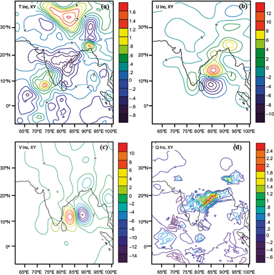
Fig. 1 Analysis increment in (a) temperature (in K), (b) u-wind (in m s-1) (c) v-wind (in m s-1), and (d) moisture (in kg kg-1) after assimilation of satellite vdata at 00:00 UTC on May 16, 2020.
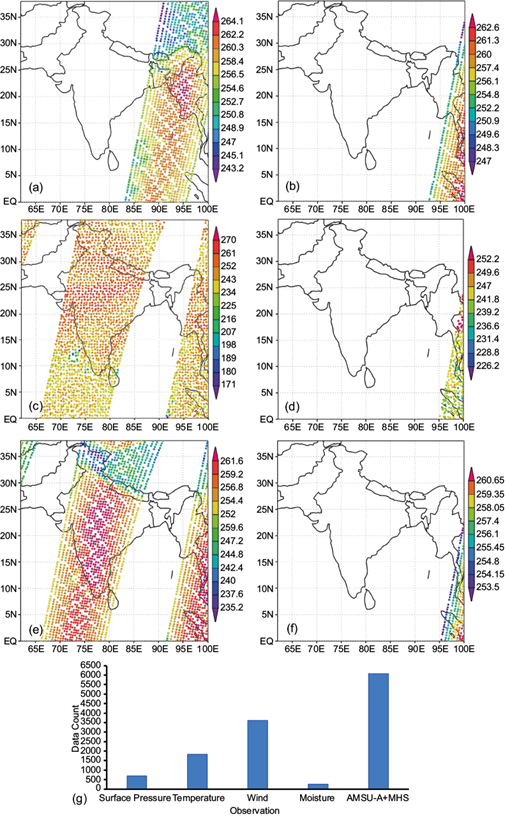
The analysis increment of the initial temperature varies from -0.8 to 1.6 K; u- and v-wind vary from -10 to 12 m s-1 and -14 to 10 m s-1, respectively, and moisture varies from -0.6 to 2.4 kg kg-1. Figure 1a shows a positive increment in temperature near the Kolkata-Bangladesh region and south of the AS region. There is a positive analysis increment in u-wind over the northern BoB and a negative analysis increment over the southern BoB, as shown in Figure 1b. Similarly, there is a positive analysis increment in the southwestern region of thr BoB, and a negative analysis increment in the region between 85º E to 95º E over the central BoB was observed for v-wind (shown in Fig. 1c). The positive analysis increment is also noted for the moisture field (around 2.4 kg kg-1) around the eastern coast of India near to the cyclonic region (shown in Fig. 1d). Figure 2a-f gives an example of the spatial distribution of satellite observations from AMSU-A and MHS in different platforms. Figure 2g shows the total conventional and satellite observations used for the assimilation at 00:00 UTC on May 16, 2020, for SuCs Amphan.
4.2 Impact on track simulation
A quantitative analysis of the impact of satellite DA was carried out on the track simulation of SuCS Amphan by considering five different ICs. Figure 3a illustrates the first simulated track from both the CTL-run and EXP-run for 72-h, generated from the IC at 00:00 UTC on May 16, 2020, for SuCS Amphan, along with the IMD best track position. Both tracks follow the same path initially up to 48 h of simulation; thereafter, a slightly northwestern movement can be observed in EXP-run with respect to the IMD’s best track. It was also observed that the CTL run moved faster than the EXP run and produced a large error. If we compare the simulated track error, it is observed that the errors in CTL-run (60, 44.7, 113.9, 96.9, 131.2, and 88.5 km) are larger compared to EXP-run (53.5, 16.4, 87.1, 54.9, 88.1, and 71 km) for the lead times of 12 to 72 h (Fig. 4 a).
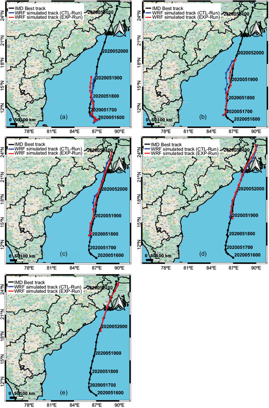
Fig. 3 Simulated tracks from CTL-run and EXP-run for (a) 72 h from the IC at 00:00 UTC on May 16, 2020, (b) 72 h from the IC at 00:00 UTC on May 17, 2020, (c) 72 h from the IC at 00:00 UTC on May 18, 2020, (d) 60 h from the IC at 00:00 UTC on May 19, 2020, and (e) 36 h from the IC at 00:00 UTC on May 20, 2020, along with IMD’s best track for SuCS Amphan.
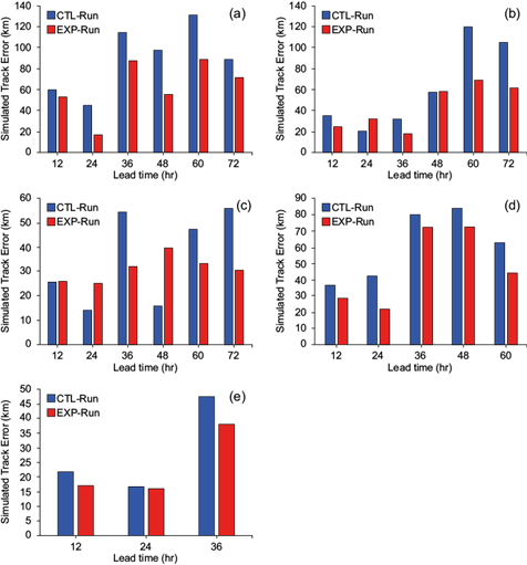
Fig. 4 Simulated track errors (in km) of CTL-run and EXP-run with respect to the IMD best track for (a) 72 h from the IC at 00:00 UTC on May 16, 2020, (b) 72 h from the IC at 00:00 UTC on May 17, 2020, (c) 72 h from the IC at 00:00 UTC on May 18, 2020, (d) 60 h from the IC at 00:00 UTC on May 19, 2020, and (e) 36 h from the IC at 00:00 UTC on May 20, 2020, for SuCS Amphan.
The second simulation was performed from 00:00 UTC on May 17, 2020. Figure 3b shows that even though both tracks have the same path until the 24-h simulation, the EXP-run track was subsequently found near the best track as compared to CTL-run. Furthermore, Figure 4b exhibits the CTL-run track error as 35, 20, 31.9, 57.7, 119.9, and 105.2 km, and the track error associated with EXP-run as 24.6, 32.2, 17.5, 58.1, 69.1, and 61.3 km for 12 to 72 h. Thus, it is observed that except for the 24-hour lead time, the track errors for all other simulation hours are found to be less for EXP-run as compared to CTL-run. The third simulation was conducted from the IC at 00:00 UTC on May 18, 2020. Both CTL-run and EXP-run followed the same path, which was close to the IMD best track; however, the CTL-run track was slightly farther from the best track (Figure 3c) for the 36- to 42-h simulation lead time. Moreover, Figure 4c shows that the EXP-run track errors were calculated as 25.7, 24.8, 32.2, 39.8, 33.5, and 30.5 km, whereas for CTL-run the track errors were found to be 25.6, 13.9, 54.6, 15.7, 47.7, and 56.1 km for the 12- to 72-h lead times. However, at 24- and 48-h, EXP-run track errors were higher than CTL-run results, but for the rest of the simulated hours, EXP-run track errors were found to be comparatively lower than in the CTL-run.
The fourth simulation was carried out from the IC at 00:00 UTC on May 19, 2020. As illustrated in Figure 3d, both CTL-run and EXP-run were nearer and followed the same best track. Figure 4d shows that track errors are about 28.6, 22.2, 72.3, 72.6, and 44.3 km for EXP-run, and 36.8, 42.3, 80.1, 84.8, and 62.8 km for CTL-run in the 12- to 60-h lead time. Hence, in the fourth simulation, EXP-run’s track error is lower than that of CTL-run throughout all simulation hours. In the fifth simulation from the IC at 00:00 UTC on May 20, 2020, Figure 3e shows that both tracks from CTL-run and EXP-run follow the same path close to the best track. Figure 4e shows that the track error is 17.2, 16.2, and 38 km for EXP-run and 21.7, 16.6, and 47.4 km for CTL-run in the 12- to 36-h simulation. The track error analysis implies that EXP-run produced less errors compared to CTL-run for all simulation hours.
The 12-hourly average track errors for both experiments are calculated and shown in Table II. The percentage improvement in EXP-run is found to be 16.5, 18.5, 24.7, 11.8%, 35, and 34.9% for lead times ranging from 12 to 72 h. Since all percentage improvements are positive, it can be inferred that incorporating AMSU-A and MHS data into the model enhanced the track simulation for cyclone SuCS Amphan.
Table II 12-hourly average simulated track errors (km) of CTL-run and EXP-run and percentage improvement in EXP-run for SuCs Amphan from all initial conditions.
| Simulation lead time (h) | Number of simulations | Track error inbr /CTL-run (km) | Track error inbr /EXP-run (km) | Percentage of improvement in EXP-run with respect to CTL-run |
| 12 | 5 | 35.8 | 29.9 | 16.5 |
| 24 | 5 | 27.5 | 22.4 | 18.5 |
| 36 | 5 | 65.6 | 49.4 | 24.7 |
| 48 | 4 | 63.8 | 56.3 | 11.8 |
| 60 | 4 | 90.4 | 58.8 | 35.0 |
| 72 | 3 | 83.3 | 54.2 | 34.9 |
A comprehensive impact study of AMSU-A and MHS observations through 3D-var DA on the track simulation of SCS Nisarga was conducted using three separate ICs. The first simulation was carried out from the IC at 00:00 UTC on June 1, 2020. Figure 5a shows the 72-h simulated tracks for CTL-run and EXP-run, along with the best IMD track. It can be observed that initially and up to the 30 h lead time, the track from CTL-run shows a curved path, whereas EXP-run exhibits a smooth, regular track closer to the best track.
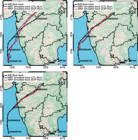
Fig. 5 Simulated tracks from CTL-run and EXP-run for (a) 72 h from the IC at 00:00 UTC on June 1, 2020 (b) 48 h from the IC at 00:00 UTC on June 2, 2020, and (c) 24 h from the IC at 00:00 UTC on June 3, 2020, along with the IMD’s best track for SCS Nisarga.
It can be observed that track errors for CTL-run in this simulation are greater (62.6, 68.7, 92.1, 106.4, 42.2, and 111.2 km) as compared to EXP-run (55.3, 61.2, 77.2, 97.6, 39.8, and 89.3 km) for lead times of 12- to 72-h, respectively (shown in Fig. 6a). Despite the initial proximity of the CTL-run track to the IMD best track, the track error of EXP-run is lower than that of the CTL-run. This is mainly because CTL-run has a time lag due to initial track diversion, resulting in larger track errors.
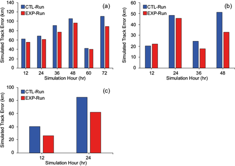
Fig. 6 Simulated track errors (in km) of CTL-run and EXP-run with respect to the IMD best track for (a) 72 h from the IC at 00:00 UTC on June 1, 2020, (b) 48 h from the IC at 00:00 UTC on June 2, 2020, and (c) 24 h from the IC at 00:00 UTC on June 3, 2020, for SCS Nisarga.
The second simulation, shown in Figure 5b, was performed from the IC at 00:00 UTC on June 2, 2020. It has been observed that both the tracks closely followed the best track up to 24 h; thereafter, the EXP-run track seems to be closer to the best track as compared to CTL-run. Further, it can be noticed that the track errors of CTL-run are found to be 20.2, 48.4, 24.4, and 51.4 km, whereas the track errors of EXP-run were calculated as 22.1, 45.6, 17.8, and 32.5 km for lead times of 12 to 48 h (shown in Fig. 6b). Consequently, except for the 12-h lead time, the track error of EXP-run is relatively lower than that of CTL-run.
Figure 5c illustrates the 24-h simulated tracks for the third simulation of CTL-run and EXP-run generated from the IC at 00:00 UTC on June 3, 2020, along with the best track of SCS Nisarga. Both CTL-run and EXP-run are found close to the best track. Moreover, Figure 6c shows that the track errors of CTL-run are about 39.43 and 84.68 km, while the track errors for EXP-run are calculated as 25.75 and 61.87 km for lead times of 12- and 24 h, respectively. This indicates that the track errors of EXP-run are relatively lower than those of CTL-run throughout all simulation hours.
The 12-hourly average track errors of both experiments are shown in Table III. The improvements in EXP-run compared to CTL-run are calculated as 15.5, 16.5, 18.5, 17.5, 5.7, and 19.7% for lead times ranging from 12 to 72 hours. These positive percentage improvements in EXP-run indicate a significant enhancement in the simulation of the SCS Nisarga’s track by incorporating AMSU-A and MHS observations into the regional model.
Table III 12-hourly average simulated track errors (km) of CTL-run and EXP-run and percentage improvement in EXP-run for SCS Nisarga from all initial conditions.
| Simulation lead time (h) | Number of simulations | Track error in CTL-run (km) | Track error in EXP-run (km) | Percentage of improvement in EXP-run with respect to CTL-run |
| 12 | 3 | 40.7 | 34.4 | 15.5 |
| 24 | 3 | 67.3 | 56.2 | 16.5 |
| 36 | 2 | 58.3 | 47.5 | 18.5 |
| 48 | 2 | 78.9 | 65.1 | 17.5 |
| 60 | 1 | 42.2 | 39.8 | 5.7 |
| 72 | 1 | 111.2 | 89.3 | 19.7 |
4.3 Impact on landfall position and time
According to the IMD, SuCS Amphan made landfall between 10:00 and 12:00 UTC on May 20, 2020, at 21.65º N and 88.3º E. Since SuCS Amphan’s landfall could be observed from the simulation starting at 00:00 UTC on May 18, 2020. the landfall position and time errors were computed from the IC at 00:00 UTC on May 18-20, 2020. A comparative analysis of the positional and temporal errors during landfall between CTL-run and EXP-run for three different ICs is presented in Tables IV-VI.
Table IV shows that the positional error during landfall is lower in EXP-run (12 km) compared to CTL-run (34.1 km). The landfall time obtained in EXP-run is also closer to the IMD observed time than in the CTL-run. Similarly, for the IC at 00:00 UTC on May 19, 2020, the error in landfall position and time in EXP-run is found to be lower than in CTL-run (shown in Tables V and VI). On May 20, 2020, the landfall time is slightly reduced, while it is found to be similar in the CTL-run. These findings indicate a significant reduction in landfall error in terms of both time and position in EXP-run for cyclone Amphan.
Table IV Landfall error estimation for SuCS Amphan based on the IC at 00:00 UTC on May 18, 2020.
| IMD observed | CTL-run | EXP-run | ||
| Landfall position | Latitude | 21.65º N | 21.90º N | 21.69º N |
| Longitude | 88.3º E | 88.12º E | 88.19º E | |
| Simulated landfall position error (km) | 34.1 | 12 | ||
| Landfall time | 10:00-12:00 UTC on May 20, 2020 | 13:00 UTC on May 20, 2020 | 12:00 UTC on May 20, 2020 | |
Table V Landfall error estimation for SuCS Amphan based on the IC at 00:00 UTC on May 19, 2020.
| IMD observed | CTL-run | EXP-run | ||
| Landfall position | Latitude | 21.65º N | 21.61º N | 21.52º N |
| Longitude | 88.3º E | 88.44º E | 88.29º E | |
| Simulated landfall position error (km) | 15.1 | 15 | ||
| Landfall time | 10:00-12:00 UTC on May 20, 2020 | 14:00 UTC on May 20, 2020 | 13:00 UTC on May 20, 2020 | |
Table VI Landfall error estimation for SuCS Amphan based on the IC at 00:00 UTC on May 20, 2020.
| IMD observed | CTL-run | EXP-run | ||
| Landfall position | Latitude | 21.65º N | 21.67º N | 21.69º N |
| Longitude | 88.3º E | 88.37º E | 88.32º E | |
| Simulated landfall position error (km) | 7.6 | 5.8 | ||
| Landfall time | 10:00-12:00 UTC on May 20, 2020 | 11:00 UTC on May 20, 2020 | 11:00 UTC on May 20, 2020 | |
The landfall time recorded by the IMD for SCS Nisarga was between 07:00 and 09:00 UTC on June 3, 2020, at 18.35º N and 72.95º E. The comparison of landfall position and time errors between CTL-run and EXP-run for three different ICs is illustrated in Tables VII, VIII and IX. The results analysis reveals a significant reduction in landfall position errors in the EXP-run simulations, while the landfall timing of both experiments is found to be close to the observed timing.
Table VII Landfall error estimation for SCS Nisarga based on the IC at 00:00 UTC on June 1, 2020.
| IMD observed | CTL-run | EXP-run | ||
| Landfall position | Latitude | 18.35º N | 18.03º N | 17.9º N |
| Longitude | 72.95º E | 72.92º E | 73.1º E | |
| Simulated landfall position error (km) | 35.49 | 52.49 | ||
| Landfall time | 07:00-09:00 UTC on June 3, 2020 | 08:00 UTC on June 3, 2020 | 08:00 UTC on June 3, 2020 | |
Table VIII Landfall error estimation for SCS Nisarga based on the IC at 00:00 UTC on June 2, 2020.
| IMD observed | CTL-run | EXP-run | ||
| Landfall position | Latitude | 18.35º N | 18.21º N | 18.22º N |
| Longitude | 72.95º E | 72.88º E | 72.91º E | |
| Simulated landfall position error (km) | 17.4 | 15.07 | ||
| Landfall time | 07:00-09:00 UTC on June 3, 2020 | 07:00 UTC on June 3, 2020 | 07:00 UTC on June 3, 2020 | |
Table IX Landfall error estimation for SCS Nisarga based on the IC at 00:00 UTC on June 3, 2020.
| IMD observed | CTL-run | EXP-run | ||
| Landfall position | Latitude | 18.35º N | 18.32º N | 18.34º N |
| Longitude | 72.95º E | 72.90º E | 72.90º E | |
| Simulated landfall position error (km) | 6.34 | 5.82 | ||
| Landfall time | 07:00-09:00 UTC on June 3, 2020 | 08:00 UTC on June 3, 2020 | 08:00 UTC on June 3, 2020 | |
4.4 Impact on the maximum sustained surface wind
The MSSW associated with a TC is a standard measure of the cyclone’s intensity. Figure 7 depicts the variation of MSSW regarding different ICs for different simulation hours for CTL-run and EXP-run in relation to the IMD-MSSW observation for SuCS Amphan.
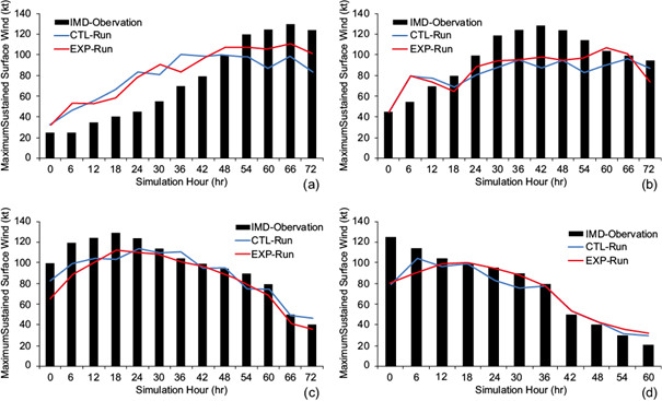
Fig. 7 Simulated MSSW values for CTL-run and EXP-run compared to IMD observed MSSW values from (a) the IC at 00:00 UTC on May 16, 2020, (b) the IC at 00:00 UTC on May 17, 2020, (c) the IC at 00:00 UTC on May 18, 2020, and (d) the IC at 00:00 UTC on May 19, 2020, for SuCS Amphan.
For the simulation at 00:00 UTC on May 16, 2020, Figure 7a shows that both CTL-run and EXP-run have overestimated the MSSW from the beginning to the 48-h lead time. Initially, the MSSW recorded from IMD observations was 46.3 km-1, whereas CTL and EXP-run estimated it as 59.1 km h-1. Subsequently, beyond the 48-h lead time, it was noted that the EXP-run MSSW plot closely aligned with the IMD observation compared to the CTL-run. Figure 7b illustrates the simulation from the IC at 00:00 UTC on May 17, 2020. After a 12-h lead time, EXP-run MSSW values are observed to be closer to IMD observations as compared to the CTL-run. Figure 7c shows the MSSW values for another simulation conducted from the IC at 00:00 UTC on May 18, 2020. It is observed that both CTL-run and EXP-run underestimated the MSSW values until the 30-h lead time, after which the EXP-run MSSW plot exhibited a smoother trend relatively closer to the IMD MSSW observations as compared to the CTL-run. Figure 7d illustrates the MSSW value from the simulation form the IC at 00:00 UTC on May 19, 2020; after a 12-h lead time, the EXP-run MSSW values were found to be more closely aligned with IMD MSSW observations as compared to the CTL-run. Figure 7 shows that during the initial simulation hours, there is a deviation in both CTL-run and EXP-run from the IMD observations, mainly due to the model’s spin-up time (Jerez et al., 2020).
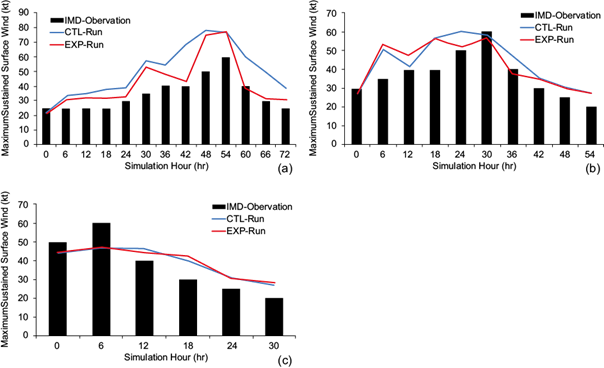
Figure 8 shows the variations of MSSW under different ICs across simulation hours in CTL-run and EXP-run, along with the IMD MSSW observation for SCS Nisarga. For the simulation initialized at 00:00 UTC on June 1, 2020, both runs initially underestimated the MSSW (Fig. 8a); however, the EXP-run’s MSSW plot exhibits a similar trend and aligns more closely with the IMD observation compared to the CTL-run. Moving on to Figure 8b, which represents the simulation initialized at 00:00 UTC on June 2 , 2020, it is evident that within the first 24 h, there is minimal disparity between the MSSW values of CTL-run and EXP-run. Nonetheless, beyond the 24-h lead time, the MSSW values in EXP-run tend to closely resemble the IMD MSSW observations compared to CTL-run. At the 30-h simulation, the EXP-run adequately captured the peak of MSSW. Subsequently, the simulation initialized at 00:00 UTC on June 3, 2020, is illustrated in Figure 8c. It is noted that both CTL-run and EXP-run initially underestimated the MSSW until the 12-h mark, after which EXP-run’s MSSW plot displays a smoother trend and aligns relatively closer to the IMD MSSW observations when compared to CTL-run.
4.5 Impact on central pressure
Intensity is often linked to central pressure (CP). Typically, a lower CP corresponds to an intense cyclone. Changes in CP indicate whether a cyclone is intensifying or weakening. Therefore, accurate CP estimations from the model are also important. Further, the model-simulated CPs are validated against the IMD-observed CP. Figure 9 shows CP variations with respect to different simulation hours at different ICs for SuCS Amphan. In Figure 9a, the simulation from the IC at 00:00 UTC on May 16, 2020, it is that both CTL-run and EXP-run initially underestimated the IMD observation. However, after an 18-hour lead time, the EXP-run plot was found to be closer to the IMD observation compared to the CTL-run. Similarly, from the IC at 00:00 UTC on May 17, 2020, as indicated in Figure 9b, the EXP-run CP value approaches the IMD perceived value more closely than the CTL-run, starting from a 12-h lead time. Nevertheless, both experiments underestimated the value compared to the IMD observation until 54 h of lead time.
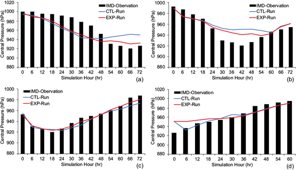
Fig. 9 Simulated central pressure values from CTL-run and EXP-run compared to IMD observed central pressure values from (a) the IC at 00:00 UTC on May 16, 2020, (b) the IC at 00:00 UTC on May 17, 2020, (c) the IC at 00:00 UTC on May 18, 2020, and (d) the IC at 00:00 UTC of May 19, 2020, for SuCS Amphan.
For the simulation initialized at 00:00 UTC on May 18, 2020, Figure 9c reveals a slight disparity between CTL-run and EXP-run initially up to the 24-h lead time. However, in subsequent simulation hours, the EXP-run plot tends to align more closely with the IMD CP values than the CTL-run values. Furthermore, for the simulation at 00:00 UTC on May 19, 2020, Figure 9d shows that both CTL-run and EXP-run initially overestimated the CP value; however, after a 24-h lead time, the EXP-run plot is closer to the IMD observation than the CTL-run.
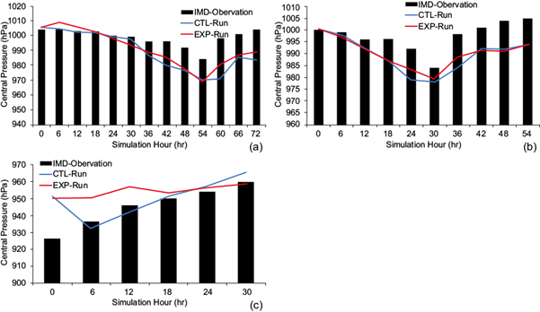
Figure 10 shows the CP variation at different ICs for SCS Nisarga. In the simulation from the IC at 00:00 UTC on June 1, 2020, shown in Figure 10a, it is evident that CTL-run and EXP-run initially exhibited values of 1005.5 and 1005.4 hPa, respectively. However, after 18 h of simulation, EXP-run CP values align more closely with the IMD observation compared to the CTL-run. Moreover, the decrease in CP at a lead time of 54 h is well depicted in the EXP-run, close to the IMD CP observation. Similarly, for the simulation at 00:00 UTC on June 2, 2020, Figure 10b shows that the EXP-run CP value is in closer agreement with the IMD observed value than CTL-run. Additionally, the decrease in CP at the 30-h simulation lead time is more accurately represented in EXP-run compared to CTL-run. For the simulation at 00:00 UTC on June 3, 2020, Figure 10c shows a slight peak at the 12-h simulation, as observed by the IMD, which is well captured by EXP-run compared to CTL-run. Furthermore, the overestimation of low pressure displayed in the CTL-run plot at the 6-h simulation is effectively reduced in EXP-run.
4.6 Impact on rainfall simulation
SuCs Amphan made landfall between 10:00 and 12:00 UTC on May 20, 2020. The rainfall linked with the Amphan cyclone during its landfall was compared to the IMERG observed rainfall. The 72-h rainfall simulations were carried out by both CTL-run and EXP-run from IC 00:00 UTC on May 17, 2020.
Figure 11a illustrates the daily accumulated rainfall (DAR) observation by IMERG on May 20, 2020, while Figure 11b, c shows the 72-h simulated DAR by CTL-run and EXP-run, valid on the same day. Both experiments exhibit a well-simulated rainfall pattern in the TC region, with the highest daily rainfall rate (≥ 64 cm day-1) matching with the observed IMERG value. Rainfall in east India is accurately represented in EXP-run (Fig. 11c) compared to CTL-run (Fig. 11b), aligning with the observed IMERG rainfall (Fig. 11a). As a result, the rainfall values over the Odisha coast are significantly improved in EXP-run. Moreover, overestimation of rainfall is observed in CTL-run within the cyclonic region of BoB, which is properly addressed by EXP-run with values close to the observed IMERG rainfall.
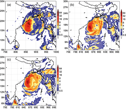
Fig. 11 (a) Daily accumulated rainfall (cm day-1) from IMERG on May 20, 2020, and 72-h simulated rainfall (cm day-1) from (b) CTL-run and (c) EXP-run, valid on May 20, 2020, for SuCS Amphan.
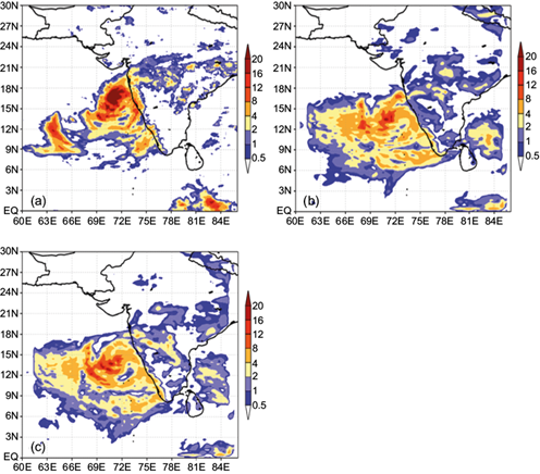
The DAR for June 2, 2020, related to SCS Nisarga, was estimated and compared with the observed DAR from IMERG. Simulations for both CTL-run and EXP-run scenarios were conducted from the IC at 00:00 UTC on June 1, 2020. Figure 12a shows the DAR observed by IMERG on June 2, 2020, while Figure 12b, c displays the 48-h simulated DAR by CTL-run and EXP-run, valid on the same day. Both experiments accurately simulate the rainfall pattern in the TC region, with the IMERG measured values matching the highest rainfall rate (≥ 20 cm day-1). The rainfall distribution in the southwest coastal area of India is accurately represented in both CTL-run and EXP-run; however, CTL-run displays an overestimated rainfall at the southern tip of India, which is well addressed by the EXP-run. Furthermore, rainfall in the latitude range from 12º to 21º N is better depicted in the EXP-run compared to the CTL-run, which matches the IMERG observed rainfall values (Fig. 12a). Moreover, CTL-run rainfall shows underestimation in the cyclonic region over the AS, and closely matches the IMERG observed DAR on 2 June 2020.
5. Conclusions
The present study evaluated the impact of assimilating AMSU-A and MHS satellite data using a 3D-var scheme on simulations of SuCs Amphan and SCS Nisarga that formed in 2020 over the BoB and AS, respectively. The assessment included analyzing the impact on the track, landfall timing and location, MSSW, CP, as well as the associated rainfall. The ARW-WRF model was employed for the simulations, while GSI with the 3D-var DA scheme was implemented to incorporate conventional and satellite observations. The model was configured with moving nested domains, with resolutions of 27 and 9 km for the parent and nested domains, respectively.
Two experiments were conducted, namely CTL-run and EXP-run. The CTL-run incorporates conventional observations, while the EXP-run assimilates both conventional observations and satellite data. TC’s track and landfall errors were assessed and compared to the IMD’s best track for both experiments. Furthermore, TC-associated simulated parameters, such as MSSW, CP, and rainfall from CTL-run and EXP-run were validated against IMD observations and precipitation observations from IMERG.
Track errors for SuCs Amphan were improved by 16.5, 18.5, 24.7, 11.8, 35, and 34.9% for EXP-run compared to CTL-run in 12-72 hours lead times. Similarly, for SCS Nisarga, improvements in track errors were improved by 15.5, 16.5, 18.5, 17.5, 5.7, and 19.7% for EXP-run for the same lead times. The consistent positive percentage improvements in EXP-run compared to CTL-run indicate that the track errors in EXP-run were reduced for lead times of 12 to 72 h. Furthermore, the landfall position errors in EXP-run (12, 15, and 5.8 km) were smaller than in CTL-run (34.1, 15.1 and 7.6 km) during May 18-20, 2020, for SuCs Amphan. Similarly, during June 01-3, 2020, the landfall position errors in EXP-run for SCS Nisarga (52.49, 15.07, and 5.82 km) were lower compared to CTL-run (35.49, 17.40, and 6.34 km), except for the first simulation. Additionally, the landfall timing in the EXP-run showed slight improvement for cyclone Amphan, whereas for cyclone Nisarga, both experiments closely matched the observed timing. EXP-run outperformed CTL-run in the case of both MSSW and CP. The rainfall patterns of Amphan and Nisarga were adequately captured, with a better representation in EXP-run than in CTL-run, especially over the cyclonic region.
In the present study, we selected two TCs that affected the Indian region as case studies. The analysis of results reveals significant improvements in regional NWP performance for TC simulation. However, to obtain more robust results, additional experiments with multiple TCs would be beneficial.
In conclusion, this study shows significant improvement in TC simulation by assimilating AMSU-A and MHS observations using the 3D-var DA technique. However, in 3D-var, the background error covariance matrix is typically static, meaning it does not change over time or adapt to the flow of the system. This can lead to uncertainty in assimilation results, especially in situations where the system dynamics are complex and highly variable. Future research could explore advanced DA techniques, such as hybrid DA, which would help to address these challenges.

