


 nueva página del texto (beta)
 Inglés (pdf)
 Artículo en XML
 Referencias del artículo
 Enviar artículo por email
 Citado por SciELO
  Similares en
SciELO
Similares en
SciELO 
 Permalink
1. Introduction
The need for meticulous planning in water resource conservation and utilization is underscored by rapid population growth and adverse environmental conditions (Aktürk and Yıldız , 2018; Tayyab et al., 2019; Ali and Shahbaz, 2020; Obasi et al., 2020). In hydrology, predictive modeling using flow data from water basins has demonstrated significant potential (Sun et al., 2019; Adnan et al., 2020). However, the nonlinear nature of hydrological data, including flow data, presents challenges in calculations and modeling (Kumar et al., 2019). Previous research commonly employs observed rainfall and runoff data to estimate output values using flow data (Singh et al., 2018; Turhan et al., 2019; Vidyarthi et al., 2020). Lake Urmia, situated in Iran’s north-western region, has experienced a substantial decrease in water level, dropping by up to 5 m in the last 45 years, attributed to factors such as climate change, overexploitation of water resources, dam construction, and reduced rainfall in the lake basin (Hassanzadeh et al., 2012). The outflow of rivers into the lake is pivotal in disrupting the stability of inflow and outflow. Predicting river inflow necessitates extensive studies to forecast rainfall levels over the basin in the coming years. However, the hydrological complexity makes it challenging to understand the correlation between rainfall and runoff (Wang et al., 2013). The R-R model, pivotal in accurately modeling rain-runoff relationships, presents a significant challenge with wide-ranging applications in water resource management, hydropower generation, irrigation, urban planning, and agrohydrological/meteorological activity planning (Alizadeh et al., 2017). To address the limitations of traditional time series models, a new class of regression models based on machine learning techniques has emerged, including Support Vector Machine (SVM), Random Forest (RF), Boosted-Tree (BT), and Multivariate Adaptive Regression Splines (MARS) (Kisi and Parmar, 2016). Park and Markus (2014) and Meng et al. (2016) identified three common models for modeling the relationship between rainfall and runoff: conceptual models, physically grounded models, and black box models. As defined by Lee et al. (2005), a conceptual model represents a network of concepts used to estimate, recreate, or understand the subject being modeled. Physically based models, as described by Calver (1988), are physical replicas of objects used to study hydrological processes. According to Kan et al. (2016), black box models are systems that allow for interrogating their inputs and outputs without requiring knowledge of their internal workings. Conceptual and physically grounded models are widely regarded as the most suitable approaches for understanding the relationship between rainfall and runoff.
Machine learning and modern approaches have gained significant traction in water resources studies, with RF and BT algorithms emerging as crucial methods for making multiple predictions. RF, an ensemble model composed of numerous BTs, has found widespread application in various fields, including environmental and water resource management (Breiman, 2001; Norouzi et al., 2018). Additionally, the BT approach, particularly for the regression model, has demonstrated efficiency in ecological modeling within hydrological regions (Nylén et al., 2014). Lee et al. (2017) conducted a study on spatial flood vulnerability prediction in metropolitan Seoul, Korea, employing RF and BT models. The RF model achieved validation accuracies of 78.78% for the regression algorithm and 79.18% for the classification algorithm, while the BT model attained validation accuracies of 77.55 and 77.26%, respectively. In the literature, several studies have applied machine learning methods in rainfall-runoff modeling in the Urmia Lake basin. Farajzadeh et al. (2014) compared monthly rainfall and runoff modeling in the Lake Urmia basin using two approaches: the “feed-forward neural network” and the “time series analysis” model. They calculated the runoff coefficient regime based on parallel rainfall data over the basin for 39 years and predicted future runoff from the forecasted rainfall. Shiri (2019) studied prediction vs. estimation of dewpoint temperature (Tdew) by assessing the Gene Expression Programming (GEP), Multivariate Adaptive Regression Spline (MARS), and Random Forest (RF) models. This study develops Tdew models using GEP, MARS, and RF with data from six weather stations in East Azerbaijan, Iran, over 10 years. GEP models excelled in predicting Tdew at daily and weekly intervals, while MARS models, using air temperature, relative humidity, and sunshine hours, were most accurate for estimating Tdew. The study recommends MARS for estimation and highlights issues with using single data sets for analysis. Asadi et al. (2019) utilized data-driven models based on artificial neural networks (ANNs) to estimate monthly runoff, achieving improved accuracy by incorporating hydrogeomorphic and biophysical time series inputs. Li et al. (2020) investigated the impact of forest change on annual runoff estimation using a statistical approach based on RF, revealing varied increases in the projected runoff across catchments. Karimi et al. (2020) surveyed supplanting missing climatic inputs in classical and RF models for estimating reference evapotranspiration in humid coastal areas of Iran. This study evaluates the impact of estimated meteorological variables on the accuracy of the Penman-FAO-Monteith (PFM) equation and empirical evapotranspiration (ETo) models. It uses 10 years of daily data from six humid coastal locations in Iran. The study finds that replacing missing inputs with estimated values improves accuracy, especially when estimated wind speed values are used. However, using estimated solar radiation values can reduce model accuracy.
Additionally, the study compares these results with machine learning models, specifically bootstrap aggregating-based RF under the same conditions. Tariq et al. (2021) explored the application of machine learning techniques for rainfall-runoff modeling in the Soan river basin in Pakistan, underscoring the importance of factors such as pool characteristics, geography, and composition in influencing the outcomes of the wavelet approach. Thus, careful selection of the wavelet family, type, and decomposition degree is crucial for optimal results. In another study, Turhan (2021) compared the effectiveness of ANNs in modeling the rainfall-runoff relationship for water resources management. Focusing on the Nergizlik dam in the Seyhan sub-basin in Turkey, the study found that ANN techniques produced statistically valid conclusions in rain-runoff modeling, with the developed models being successfully applied to evaluate medium monthly runoff. Bigdeli et al. (2023) studied the application of SVM and the BT algorithm for rainfall-runoff modeling at Tabriz Plain. The results showed that, during the study periods, the SVM model outperformed the BT model at Akhula station, while the BT model performed better than SVM model for Pole Senikh station. In the last study, Bigdeli et al. (2024) surveyed rain-runoff modeling of Khormazard and Bonab hydrometric stations using SVM and RF algorithms. In this research, rainfall-runoff simulation of Khormazard and Banab stations (on Sufichai and Mahperichai rivers) was carried out using data mining models of SVM and RF models. The results showed that in the Bonab station, the SVM model had higher efficiency than the RF model, and in the Khormazard station, the latter model provided better performance than SVM model during the study periods.
The literature lacks descriptions of rainfall-runoff modeling in the Lake Urmia basin using heuristic models. This study focuses on the application and validation of RF and BT heuristic methods in the all-sub-basins of Lake Urmia, utilizing chronological records of parameters and regional-scale meteorological inputs. The significance of each variable was computed, and RF and BT models were compared. The RF and BT models were chosen for rainfall-runoff modeling in the Urmia Lake basin because these models had not been previously applied in this region. The aim is to obtain more accurate predictions of monthly discharge, prioritizing the most practical and available model based on hydrological insights. Also, this study represents the first application of RF and BT models to predict/estimate the rainfall-runoff from 16 key Lake Urmia Basin stations.
2. Methodology
2.1 Study area and data description
Lake Urmia Basin, located at 44º 07’-47º 53’ E longitude and 35º 40’-38º 30’ N latitude, is one of the six main basins of Iran, with a total size of 52 679 km2. The basin encompasses 34 000 km2 of mountainous terrain and 13 000 km² of flat terrain, with 6000 km2 dedicated to arable land and orchards. The remaining 5000 km2 of the basin is occupied by Lake Urmia, which is considered a huge water body in Iran. Figure 1 shows the Lake Urmia basin along with its river network and hydrometric stations. Daily, monthly, and yearly rainfall and runoff data were provided by two Iranian institutions: the Iran Meteorological Organization and the Regional Water Company of East Azerbaijan. This data, spanning 43 years (1976-2019), was collected from 228 rain gauge stations within and around the lake and from 16 major runoff gauge stations leading into the Lake Urmia basin. The selected stations for our study were Akhula, Daryan, Pole Senikh, Shishvan, Gheshlagh Amir, Ghermez Gol, Shirin Kandi, Khormazard, Miandoab, Pole Ozbak, Babarud, Aghjalu Sofla, Yalghoz Aghaj, Keshtiban, Pole Bahramlu, and Nezam Abad, which are the final ones before the water reaches Lake Urmia, and no further water is collected beyond these points (see Fig. 1).
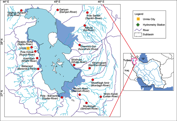
The Urmia Lake basin contains 228 rain gauge stations and 16 hydrometer stations. In this research, 16 selected stations leading to Lake Urmia were used. The characteristics of the selected stations for rainfall and discharge in the study basin are presented in Table I.
Table I Characteristics of the studied stations in the Urmia Lake basin.
| Station | River | Average rainfall (mm) |
| Akhula | Aji chai | 235.7 |
| Daryan | Daryan chai | 341 |
| Pole Senikh | Senikh chai | 203.9 |
| Ghermez gol | Azarshahr chai | 355 |
| Khormazard | Mahpari chai | 307.1 |
| Shishvan | Ghale chai | 276.9 |
| Shirin kandi | Leilan chai | 307.1 |
| Gheshlagh Amir | Mordagh chai | 345.7 |
| Miandoab | Simine Rud | 358.4 |
| Babarud | Barandoz chai | 363.1 |
| Keshtiban | Shar chai | 315.3 |
| Pole Ozbak | Roze chai | 263 |
| Abajalu Sofla | Nazlo chai | 270.3 |
| Yalghoz Aghaj | Zola chai | 171 |
| Nezam Abad | Zarine Rud | 258.7 |
| Pole Bahramlu | Godar chai | 251.6 |
2.2 Equivalent rainfall computed via the Thyssen polygons
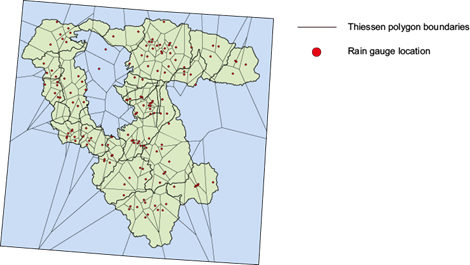
Thiessen polygons, also known as Voronoi cells (Aurenhammer et al., 2013), are utilized to identify the respective rainfall polygon for the surface. These polygons are employed to calculate the rainfall weight for each rain gauge (r i ). They also aid in determining the equivalent rainfall polygon for the area (A i ), enabling the weighing of the rainfall measurements from each rain gauge (r i [t]). Then, the equivalent area-weighted rain is obtained as
The GIS software used to describe the geographic parameters of the watershed is typically used to compute Eq. (1). As shown in Figure 2, the relevant Thiessen polygons were generated with Quantum GIS 0.8 (www.qgis.org) (Shekar and Xiong, 2007; Petrasova et al., 2015), and the equivalent rainfall was calculated with Eq. (1).
2.3 Theory
2.3.1 The Random Forest (RF) model
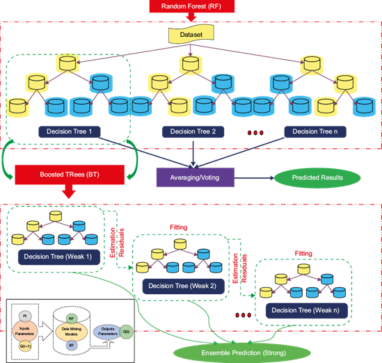
RF is a machine-learning model based on decision trees. It has been widely employed for solving classification and regression tasks. In this study, the RF algorithm is used as a regression approach to construct a predictive model for a continuous variable. The RF regression technique generates n data sets of random samples from the original data set using bootstrapping. The new datasets are then used to build n trees, ensuring that each boosted tree in the model is generated using a random subset. As a result, n trees (number of trees), N features (number of random predictors used at each node to construct each tree), and tree depth (number of nodes in each tree) act as hyperparameters that optimize the achieved model using a grid search approach that currently ranks all possible RF models using the OOB score. In RF modeling, three parameters require definition: (1) the number of trees to be grown in the forest (n tree ), which is a crucial parameter for RF; (2) the number of predictor variables randomly chosen at each node (m try ), and (3) the minimum number of observations needed at the terminal nodes of the trees (node size) (refer to Fig. 3).
2.3.2 Boosted-Tree (BT) model
The BT approach is part of a larger class of stochastic grade boosting algorithms comprehended as Tree Net (TM Salford Systems,) and MART (TM Jerill). Recently, this approach has emerged as a highly effective tool for data mining and predictive modeling. These robust algorithms are capable of handling both regression and classification tasks involving continuous and categorical variables (Friedman et al., 2013). The BT approach has been widely used for solving regression problems, particularly for predicting continuous dependent variables. However, when dealing with a large number of classes, the analysis of categorical dependent variables can become less accurate due to the potential need for significant effort and time. Similar to the RF algorithm, the BT algorithm is an ensemble learning approach that considers the performance of previous classifiers for classification and regression tasks. In the case of regression, BTs are developed from prediction residuals of the previous tree, and the basic concept is to create a set of simple trees. However, as the complexity of the trees increases, there may be issues with overfitting, where the algorithm builds a model that is overly specialized to the input data. This can be a consideration when using BT techniques in regression problems.
Both the RF and BT algorithms employ an ensemble learning strategy by constructing multiple decision trees. The RF method randomly selects data from the input dataset to build individual decision trees, which are then aggregated to form the final model, with tree weights determined based on performance (Breiman, 2001). Conversely, the BT approach also selects random data from the input dataset, similar to RF, but constructs a BT by iteratively building trees that correct the errors of the previous ones, thereby enhancing model accuracy (Naghibi et al., 2016; Tan et al., 2016). RF and BT differ in how they incorporate the classification history of previous iterations during the sample extraction and model development process. Figure 3 outlines the general algorithms of RF and BT, along with the methodology flowchart.
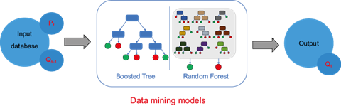
The analysis and modeling of rainfall-runoff relationships used monthly data from 228 stations inside and outside the Urmia Lake basin, along with monthly flow data from 16 hydrometric stations surrounding the lake. Three input scenarios were created to evaluate the impact of time lags and past rainfall-runoff relationships on forecast performance: (1) current monthly flow from 13 tributaries of Lake Urmia and 16 hydrological stations in the sub-basins; (2) monthly discharge data from the 16 stations between the current month (t) and the previous month (t-1). The optimal time lag for predicting the rain-runoff model, considered the most sensitive parameter, was determined through trial and error. The dataset was divided into 70% test data and 30% validation data for each model, with random selection for training and testing. Data processing methods are detailed in Figure 3. RF and BT models were compared using different runoff and rainfall data combinations, with runoff as the target variable and rainfall as the predictor variable. Inputs included previous monthly runoff (Q t-1 ) and rainfall (P t ) values, while the output represented current runoff data (Q t ). Various input combinations were evaluated, and both RF and BT models were used to identify the optimal combination (as depicted in Table II and Fig. 4). Using the modeling, the amount of current runoff was obtained with current rainfall and previous runoff. The time lag exists because the model, in addition to the current data, also pays attention to the past data to increase the accuracy of the prediction. In this study, the following hyper-parameters were used for the RF and BT models:
RF: The model was configured with 200 trees and a maximum tree depth of 10 to prevent overfitting. The minimum number of samples required to split a node was set to five, and at least two samples were required for a leaf node. Additionally, the number of features considered for each split was set to the square root of the total features, and bootstrap sampling was enabled.
BT: For the BT model, 300 boosting rounds were used, with a learning rate of 0.1 to balance model accuracy and training speed. The maximum depth of each tree was set to five, with a minimum of 10 samples required to split a node. A subsample ratio of 0.8 was used to control overfitting, and the model utilized 80% of the features for each tree.
Table II Input combination of runoff (Q) and rainfall (P) data.
| No | Model | Input | Output |
| 1 | RF | P t , Q t-1 | Q t |
| 2 | BT | P t , QQ t-1 | Q t |
Rainfall and flow data from 1976 to 2019 were collected and used as training and validation data for these data mining methods. The models were applied using the statistical tool Statistica 12, ArcGis 10.3, Matlab 2021, and Grapher 20.2 to draw graphs. The Iran Meteorological Organization and the Regional Water Company of East and West Azerbaijan provided the necessary parameters for analyzing the relationship between rainfall and runoff in this study. Subsequently, the RF and BT models were implemented, and the results were compared. The rainfall-runoff connection was studied in the following ways: (1) information was collected, associated parameters were collected and calculated; (2) spatial datasets were constructed in raster format; (3) the RF and BT models were utilized to study the relationship between rainfall and runoff, and the significance values of each predictor were computed during the course of the study; and (4) The rainfall-runoff data were used to validate the susceptibility from 1976.
2.4 Performance criteria
The performance of the RF and BT approaches was evaluated using various criteria, which included root mean square error (RMSE), Pearson correlation coefficient (r), determination coefficient (R2), and Nash-Sutcliffe efficiency (NSE) (Lan, 2014). The R2 value was utilized to measure the linear relationship between observed and estimated rain and runoff amounts, with values exceeding 1 indicating superior prediction and 1 representing excellent prediction. The RMSE assessed the goodness of fit for high rainfall-runoff values, with lower RMSE values indicating better forecast performance and a value of 0 suggesting excellent prediction (Hamidi et al., 2015). Moreover, the efficiency coefficient was employed to compare the variability of observed rainfall and runoff values with the differences between observed and estimated values. In this research, cross-correlation (CC), R², NSE, and RMSE are widely used in hydrological modeling to assess model performance from different perspectives. Together, these metrics provide a comprehensive evaluation of the model’s accuracy.
RMSE: due to its sensitivity to outliers in the data set, this measure may be prone to errors when simulating high flow rates (Dawson et al., 2006):
Pearson correlation coefficient (r):
R-squared (R2): the strength of the relationship between the observed and simulated time series is quantified by the coefficient of determination (R2), which ranges from 0.0 to 1.0, with larger values indicating greater collinearity.
Nash-Sutcliffe efficiency (NSE): In the scenario of a perfect model with zero estimation error variance, the resulting Nash-Sutcliffe efficiency is equals to 1 (NSE = 1):
where P i and Q i represent the observed and modelled runoff using the developed models, respectively, while O i is the average of observed runoff, and n is number of observations.
Trend analysis, a crucial tool for assessing climate change, utilizes various methods categorized as parametric and non-parametric. While parametric tests are considered stronger in normally distributed data, non-parametric tests, such as the Mann-Kendall method, are preferable for non-normal data conditions, common in climate series like rainfall and streamflow (Pasquini, 2006; Sabouhi and Soltani, 2008). Originally proposed by Mann (1945) and further developed by Kendall (1975), the Mann-Kendall test is extensively used in hydrological and meteorological time series analysis (Lettenmaier et al., 1994; Serrano et al., 1999). Its advantages include applicability to diverse time series distributions and low sensitivity to extreme values (Turgay and Ercan, 2005). The test’s null hypothesis assumes randomness and the absence of a trend, while rejecting it indicates the presence of a trend in the data series. The Mann-Kendall test is defined by the statistic S as follows:
where X j and X i are the sorted values of the sample, and n is the number of samples.
The variance is calculated with Eqs. (8) or (9).
where n is the number of observation data and m represents the number of series in which there is at least one repeated data. It also represents the frequency of data with the same value.
The standardized score Z and the variance of the statistic S are calculated from the following equation:
Positive values of Z indicate increasing trends, while negative values of Z indicate decreasing trends. When S = 0, there is no significant or non-significant trend in the data. These conditions are rarely ideal for hydrological data. In this study, significance levels of P = 0.05 were employed.
3. Discussion and results
3.1 Results related to the time series of rainfall and runoff for the studied time period
Figures 5 and 6 show the time series data concerning the rainfall and runoff of 16 stations within the east and west regions of the Urmia basin, which align with the results obtained from the Mann-Kendall test for annual rainfall and discharge (Tables II and III). According to Table II, Kendall’s statistic for the rainfall variable at stations Akhula, Daryan, Pole Senikh, Shishvan, Gheshlagh Amir, Ghermez Gol, Shirin Kandi, and Khormazad is determined as -0.89, 1.65, 0.031, 0.77, -1.15, 1.61, -0.41 and 1.30, respectively. Similarly, the values obtained in the west sub-basin stations Miandoab, Babarud, Keshtiban, Pole Ozabk, Yalghoz Aghaj, Nezam Abad, and Pole Bahramlo are 1.18, 0.39, -2.61, -1.79, 1.13, -0.39, 0.94 and -1.42, respectively. The results indicate that annual rainfall in the period 1976-2019 is not statistically significant at the 95% level for all stations. Therefore, it can be inferred that annual rainfall at these stations during the above-mentioned period has shown no significant trend, with natural variations occurring during this period. The data exhibit oscillatory behavior, with some years showing increasing trends and others showing decreasing trends.
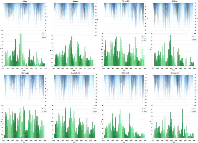
Fig. 5 Time-series plots of observed rainfall and runoff values at eight stations in the eastern sub-basin (1976-2019).
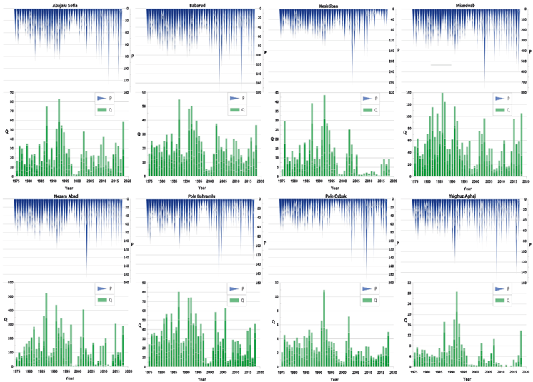
Fig. 6 Time-series plots of observed rainfall and runoff values at eight stations in the western sub-basin (1976-2019).
In addition to rainfall, the results obtained from the Mann-Kendall test indicate that the discharge from stations in both the eastern and western sub-basins of Lake Urmia exhibits a decreasing trend. In recent years, a considerable reduction in the discharge trend has been observed, posing a significant threat to Lake Urmia. Table III shows the discharge variables for eastern stations Akhula, Daryan, Pole Senikh, Shishvan, Gheshlagh Amir, Ghermez Gol, Shirin Kandi, and Khormazard, determined as -2.369, -0.35, -2.264, -1.1, -2.19, -1.82, -1.6, and -1.2, respectively. Similarly, the values obtained in the west sub-basin (Table IV) for stations Miandoab, Babarud, Keshtiban, Pole Ozabk, Yalghoz Aghaj, Nezam Abad, and Pole Bahramlo, are -2.61, -3.52, -2.75, -1.6, -2.63, -1.1, -0.69 and -0.69, respectively, indicating a statistically significant decreasing trend at the 95% confidence level. According to the results obtained from Tables III and IV, and the graphs in Figures 5 and 6, the inflow discharge into Lake Urmia has decreased at all stations during recent years, which is consistent with findings from other research and studies on the lake basin and is considered the primary reason for its declining water level (Vaheddoustand Aksoy, 2018; Hamidi-Razi et al., 2019; Lari et al., 2019).
Table III Statistical values of the Mann-Kendall test for rainfall and runoff in the eastern sub-basin (1976-2019).
| State | Station | Rainfall | Runoff |
| East Azarbaijan | Akhula | -0.89 | -2.369 |
| Daryan | 1.65 | -0.35 | |
| Pole senikh | 0.031 | -2.264 | |
| Shishvan | 0.77 | -1.1 | |
| Gheshlagh amir | -1.15 | -2.19 | |
| Ghermez gol | 1.61 | -1.82 | |
| Shirin kandi | -0.41 | -1.6 | |
| Khormazard | 1.30 | -1.2 |
Table IV Statistical values of the Mann-Kendall test for rainfall and runoff in the western sub-basin (1976-2019).
| State | Station | Rainfall | Runoff |
| West Azarbaijan | Miandoab | 1.18 | -2.61 |
| Babarod | 0.39 | -3.52 | |
| Keshtiban | -2.61 | -2.75 | |
| Pole Ozbak | -1.79 | -1.6 | |
| Abajalo Sofla | 1.13 | -2.63 | |
| Yalghoz Aghaj | -0.39 | -1.1 | |
| Nezam Abad | 0.94 | -0.69 | |
| Pole Bahramlo | -1.42 | -0.69 |
For further comparison, Figures 5 and 6 show the time series of the observed rainfall and runoff data at 16 stations over this period (1976-2019). In these charts, it can be seen that in each station, the temporal trend of rainfall shows the frequency of yearly rainfall and that in some years, it has irregularly decreased and sometimes increased. In their study’s results, Salehi et al. (2018) confirmed that the frequency of monthly rainfall events lower than 5 mm increased significantly at a 1% level in certain areas while showing no significant trend in other areas. Additionally, the area with rainfall events in the range of 10-15 mm exhibited a significant decreasing trend. Furthermore, the direction of the runoff series in the studied stations situated in the eastern and western parts of Lake Urmia showed a decreasing trend in discharge changes. Runoff figures indicate a complete decrease in lake inflow over the past 43 years, notably declining in recent years. In fact, Figures 5 and 6 confirm the results of the Mann-Kendall test presented in Tables II and III.
This decline is primarily attributed to increased local water demand and intensive agricultural development, accounting for over 60% of renewable water resource usage and 93% of total water resource utilization in the basin (Nordberg et al., 2014). According to the findings of Nazeri-Tahroudi et al. (2018), the decreasing trend in the water level of Lake Urmia was observed one year after the declining trend in the flow data. Numerous studies have been carried out to investigate trends in river flow and rainfall in the Lake Urmia basin, and all of them have confirmed that not only the water inflow to the lake has decreased, but also the water level has declined. The significant loss of water at Lake Urmia can be attributed to several factors, including: (1) construction of dams on the 13 rivers that flow into the lake, which has resulted in reduced inflows and contributed to the lowering of the lake’s water level; (2) increased groundwater pumping; (3) water diversions; (4) climate change, and (5) drought (Ahmadaali et al., 2018; Vaheddoost and Aksoy, 2018; Alizade et al., 2019; Hamidi-Razi et al., 2019; Lari et al., 2019; Marks, 2019; Bashirian et al., 2020; Hosseini-Moghari et al., 2020; Javadzadeh et al., 2020). It should be noted that in Figures 5 and 6, the unit of runoff is m3 s-1, and the unit of rainfall is mm.
To study the selected rainfall and runoff stations in the mentioned period, the rainfall and runoff statistics (average, minimum, maximum) for these years are presented in Tables V and VI, which were divided into five columns, and subsequently, the third, fourth, and fifth columns were segregated into two distinct categories or sections. The third column (total data) contains the P and Q parts. The fourth and fifth columns display the allocation of data into two separate sets: the training set and the test set. Consequently, the BT and RF models were trained and tested using real data in this study. As shown in Tables V and VI in the “total data” column, the Shishvan and Miandoab stations have the highest average rainfall. Similarly, the Akhula and Miandoab stations have the highest average runoff among the recorded events, making them the most influential in affecting the water volume of Lake Urmia. Conversely, the Pole Senikh and Abajalu Sofla stations registered the lowest average rainfall, while the Khormazard and Pole Ozbak stations showed the lowest average runoff in the study area.
Table V Statistics parameters of rainfall and runoff data and Random Forest (RF) and Boosted Tree (BT) models at eastern stations (1976-2019).
| Station | Parameter | Whole data set | Training set | Test set | |||
| P (mm month-1) | Q (m3 s-1) | BT | RF | BT | RF | ||
| Akhula | Mean Minimum Maximum | 22.22 0.00 77.66 | 7.90 0.00 92.50 | 7.68 0.00 76.85 | 8.29 0.00 76.85 | 7.49 0.00 46.29 | 6.32 0.00 47.47 |
| Daryan | Mean Minimum Maximum | 25.11 0.00 97.19 | 0.40 0.00 3.07 | 0.41 0.00 3.24 | 0.43 0.00 3.24 | 0.38 0.00 2.55 | 0.33 0.00 2.32 |
| Pole Senikh | Mean Minimum Maximum | 19.78 0.00 81.25 | 0.66 0.00 3.63 | 0.66 0.00 3.63 | 0.70 0.00 3.86 | 0.68 0.00 3.86 | 0.61 0.00 3.70 |
| Shishvan | Mean Minimum Maximum | 30.03 0.00 98.70 | 1.21 0.00 17.08 | 1.29 0.00 2.94 | 1.54 0.00 32.94 | 1.33 0.00 10.97 | 0.83 0.00 9.69 |
| Gheshlagh Amir | Mean Minimum Maximum | 26.38 0.00 91.69 | 2.16 0.01 14.97 | 2.09 1.01 14.97 | 2.32 0.01 14.97 | 2.33 0.01 13.30 | 1.83 0.01 10.60 |
| Ghermez Gol | Mean Minimum Maximum | 23.32 0.00 88.03 | 0.81 0.00 4.35 | 0.82 0.00 4.12 | 0.86 0.00 4.35 | 0.81 0.00 4.35 | 0.73 0.00 3.75 |
| Shirin Kandi | Mean Minimum Maximum | 26.69 0.00 96.73 | 1.45 0.00 º12.54 | 1.41 0.00 12.56 | 1.61 0.00 16.72 | 1.63 0.00 16.72 | 1.20 0.00 10.20 |
| Khormazard | Mean Minimum Maximum | 26.68 0.00 94.18 | 0.25 0.00 14.81 | 0.25 0.00 3.23 | 0.29 0.00 3.23 | 0.26 0.00 1.94 | 0.18 0.00 1.40 |
Table VI Statistics parameters of rainfall and runoff data and Random Forest (RF) and Boosted Tree (BT) models at western stations (1976-2019).
| Station | Parameter | Whole data set (1976-2019) | Training set | Test set | |||
| P (mm month-1) | Q (m3 s-1) | BT | RF | BT | RF | ||
| Miandoab | Mean Minimum Maximum | 128.99 0.00 755.95 | 14.92 0.00 139.63 | 14.51 0.00 115.61 | 15.84 0.00 139.63 | 15.93 0.00 139.63 | 13.32 0.00 116.39 |
| Babarud | Mean Minimum Maximum | 32.30 0.00 178.52 | 7.29 0.00 54.86 | 7.00 0.00 54.86 | 7.26 0.00 54.86 | 7.99 0.00 55.33 | 7.38 0.00 37.24 |
| Keshtiban | Mean Minimum Maximum | 39.62 0.00 290.27 | 3.07 0.00 43.65 | 2.86 0.00 39.36 | 3.08 0.00 43.65 | 3.56 0.00 43.65 | 3.06 0.00 30.51 |
| Pole | Mean Minimum Maximum | 25.10 0.00 192.57 | 1.04 0.00 10.98 | 0.98 0.00 6.62 | 1.05 0.00 10.98 | 1.18 0.00 10.98 | 1.01 0.00 10.64 |
| Abajalu Sofla | Mean Minimum Maximum | 22.96 0.00 126.28 | 6.65 0.00 83.12 | 6.41 0.00 74.94 | 6.52 0.00 83.12 | 7.27 0.00 83.12 | 6.97 0.00 58.52 |
| Yalghoz Aghaj | Mean Minimum Maximum | 27.02 0.00 156.41 | 1.48 0.00 28.62 | 1.30 0.00 18.07 | 1.46 0.00 28.62 | 1.88 0.00 28.62 | 1.52 0.00 20.96 |
| Nezam Abad | Mean Minimum Maximum | 32.97 0.00 186.96 | 41.89 0.00 523.92 | 39.09 0.10 440.58 | 43.30 0.04 523.92 | 48.20 0.01 523.92 | 38.94 0.01 320.99 |
| Pole Bahramlu | Mean Minimum Maximum | 25.69 0.00 167.52 | 9.55 0.00 80.31 | 9.06 0.00 80.31 | 9.52 0.00 80.31 | 10.75 0.00 74.37 | 9.67 0.00 62.88 |
In this section, the validation process of the optimal BT and RF models is presented to showcase their ability to model the rainfall-runoff relationship. Tables VII and VIII present the validation statistics of each optimal model for all stations over the eastern and western sub-basins of Urmia Lake in the period (1976-2019).
Table VII Performance of the Random Forest (RF) and Boosted Tree (BT) models in the training and testing sets over the eastern sub-basin (1976-2019).
| Station | Whole data set | CC | R2 | NSE | RMSE | ||||
| BT | RF | BT | RF | BT | RF | BT | RF | ||
| Akhula | Train Test | 0.87 0.81 | 0.85 0.82 | 0.76 0.65 | 0.73 0.67 | 0.76 0.65 | 0.72 0.66 | 6.10 6.05 | 6.77 5.43 |
| Daryan | Train Test | 0.87 0.78 | 0.87 0.80 | 0.75 0.61 | 0.76 0.64 | 0.75 0.61 | 0.75 0.63 | 0.26 0.28 | 0.27 0.22 |
| Pole Senikh | Train Test | 0.81 0.77 | 0.80 0.66 | 0.66 0.59 | 0.64 0.44 | 0.66 0.59 | 0.63 0.44 | 0.41 0.47 | 0.45 0.50 |
| Shishvan | Train Test | 0.90 0.75 | 0.81 0.70 | 0.82 0.56 | 0.65 0.48 | 0.79 0.51 | 0.53 0.44 | 1.53 1.66 | 2.49 1.23 |
| Gheshlagh Amir | Train Test | 0.86 0.80 | 0.90 0.77 | 0.74 0.64 | 0.81 0.60 | 0.74 0.64 | 0.80 0.58 | 1.31 1.70 | 1.26 1.37 |
| Ghermez Gol | Train Test | 0.87 0.74 | 0.91 0.84 | 0.76 0.54 | 0.82 0.70 | 0.76 0.54 | 0.82 0.69 | 0.44 0.65 | 0.41 0.48 |
| Shirin Kandi | Train Test | 0.85 0.77 | 0.87 0.63 | 0.72 0.59 | 0.76 0.40 | 0.72 0.59 | 0.75 0.26 | 0.98 1.45 | 1.09 1.32 |
| Khormazard | Train Test | 0.73 0.71 | 0.79 0.69 | 0.54 0.51 | 0.62 0.48 | 0.53 0.51 | 0.62 0.36 | 0.27 0.26 | 0.28 0.18 |
CC: cross-correlation; R2: determination coefficient; NSE: Nash-Sutcliffe efficiency; RMSE: root mean square error.
Table VIII Performance of the Random Forest (RF) and Boosted Tree (BT) models in the training and testing sets over the western sub-basin (1976-2019).
| Station | Whole data set | CC | R2 | NSE | RMSE | ||||
| BT | RF | BT | RF | BT | BT | RF | BT | ||
| Miandoab | Train Test | 0.83 0.82 | 0.86 0.85 | 0.68 0.68 | 0.73 0.71 | 0.68 0.68 | 0.72 0.71 | 11.54 13.74 | 11.98 10.49 |
| Babarud | Train Test | 0.89 0.87 | 0.90 0.87 | 0.79 0.76 | 0.80 0.76 | 0.86 0.77 | 0.78 0.76 | 3.96 4.75 | 4.09 4.10 |
| Keshtiban | Train Test | 0.83 0.82 | 0.87 0.74 | 0.83 0.82 | 0.75 0.54 | 0.75 0.65 | 0.73 0.51 | 2.82 4.15 | 3.06 3.75 |
| Pole Ozbak | Train Test | 0.88 0.81 | 0.87 0.81 | 0.78 0.65 | 0.76 0.66 | 0.88 0.64 | 0.73 0.64 | 0.51 1.03 | 0.68 0.79 |
| Abajalu Sofla | Train Test | 0.81 0.78 | 0.83 0.83 | 0.65 0.61 | 0.69 0.69 | 0.74 0.61 | 0.67 0.67 | 6.30 8.33 | 6.97 6.57 |
| Yalghoz Aghaj | Train Test | 0.82 0.72 | 0.76 0.65 | 0.67 0.51 | 0.57 0.42 | 0.75 0.45 | 0.52 0.41 | 1.30 2.79 | 1.98 2.14 |
| Nezam Abad | Train Test | 0.81 0.81 | 0.87 0.84 | 0.66 0.66 | 0.76 0.70 | 0.73 0.61 | 0.73 0.69 | 36.59 51.74 | 38.18 32.91 |
| Pole Bahramlu | Train Test | 0.86 0.88 | 0.93 0.88 | 0.74 0.77 | 0.86 0.77 | 0.82 0.75 | 0.85 0.77 | 6.69 8.03 | 5.60 6.54 |
CC: cross-correlation; R2: determination coefficient; NSE: Nash-Sutcliffe efficiency; RMSE: root mean square error.
To select the best model for each station in the basin of Lake Urmia, statistical analyses were also performed to determine the cross-correlation between rainfall-runoff and past runoff at each station. R2, NSE, and RMSE statistics were used to evaluate this cross-correlation . The results indicated that both RF and BT models performed well in both east and west sub-basins. However, as seen in Table VII, the BT model outperformed the RF model in rainfall-runoff modeling at five out of the eight studied stations in the eastern sub-basin, while the RF model performed better at three stations. Overall, a strong correlation between rainfall and runoff parameters was observed across all stations. As outlined in Table VII, the maximum cross-correlation in the test dataset for the RF and BT models ranged from 0.71 to 0.82. The optimal model for each station varied depending on the specific characteristics of that station.
On the other hand, as shown in Table VIII, the RF model outperformed the BT model in rainfall-runoff modeling at five out of the eight studied stations in the western sub-basin, while the BT model performed better at three stations. As seen in Table VIII, the maximum cross-correlation in the test dataset for the RF and BT models ranged from 0.72 to 0.88. Overall, a strong correlation between rainfall and runoff parameters was observed across all stations in this sub-basin.
In the Akhula station, a statistical analysis comparing the RF and BT models revealed that the former exhibited higher modeling accuracy. In this station, RF yielded a CC of 0.85, R2 of 0.73, NSE of 0.72, and RMSE of 6.77 on the training dataset, and CC = 0.82, R2 = 0.67, NSE = 0.66, and RMSE = 5.43 on the test dataset. Conversely, at the Daryan station, RF yielded CC = 0.87, R2 = 0.76, NSE = 0.75, and RMSE = 0.27 on the training dataset, and CC = 0.80, R2 = 0.64, NSE = 0.63, and RMSE = 0.22 on the test dataset. At the Pole Senikh station, the CC, R2, NSE, and RMSE results on the training dataset for BT model were 0.81, 0.66, 0.66, and 0.41, respectively, and 0.77, 0.59, 0.59, and 0.47, respectively, on the testing dataset. Conversely, at the Shishvan station, the BT model outperformed the RF model, with CC values of 0.90 on the training dataset, and 0.75 on the testing dataset, respectively. Similarly, at the Gheshlagh Amir station, the BT model exhibited better performance, with CC values of 0.86 on the training dataset and 0.80 on the testing dataset, respectively. Also, at the Ghermez Gol station, the RF model performed better than BT, achieving a CC = 0.91, R2 = 0.82, NSE = 0.82, and RMSE = 0.41 on the training dataset, and CC = 0.84, R2 = 0.70, NSE = 0.69, and RMSE = 0.48 on the testing dataset. At the Shirin Kandi station, the BT model outperformed the RF model, with CC values of 0.85 on the training dataset and 0.77 on the testing dataset, respectively. Similarly, at the Khormazard station, the BT model demonstrated a stronger relationship between rainfall and runoff compared to the RF model. The CC values were 0.73 on the training dataset and 0.71 on the testing dataset, respectively.
Notably, in the Akhula station, the BT model exhibited higher CC coefficients in the training data compared to the RF model. However, this higher performance in training data did not translate to better accuracy in the test dataset, suggesting overfitting. Consequently, the RF model, which performed well in both training and testing, was selected as the superior model. Conversely, at the Gheshlagh Amir, Shirin Kandi, and Khormazard stations, the RF model was overfitted, leading to inferior performance compared to BT, thus making this model the preferred choice.
On the other hand, Table VIII shows that at the Miandoab station, the RF model exhibited higher accuracy in modeling compared to BT. In this station, RF achieved a CC of 0.86, R2 of 0.73, NSE of 0.72, and RMSE of 11.98 on the training dataset, and CC = 0.85, R2 = 0.71, NSE = 0.71, and RMSE = 10.49 on the test dataset. Conversely, at the Babarud station, BT yielded a CC = 0.89, R2 = 0.79, NSE = 0.86, and RMSE = 3.96 on the training dataset, and CC = 0.87, R2 = 0.76, NSE = 0.77, and RMSE = 4.75 on the test dataset. At the Keshtiban station, the CC, R2, NSE, and RMSE results on the training dataset for the BT model were 0.83, 0.83, 0.75 and 2.82, respectively, and 0.82, 0.82, 0.65, and 4.15, respectively, on the testing dataset. Also, at the Pole Ozbak station, the RF model outperformed the BT model, with CC values of 0.87 on the training dataset, and 0.81 on the testing dataset, respectively. Similarly, at the Abajalu Sofla station, the RF model exhibited better performance, with CC values of 0.83 on the training dataset, and 0.83 on the testing dataset. Also, at the Yalghoz Aghaj station, the BT model performed better than RF, achieving a CC = 0.82, R2 = 0.67, NSE = 0.75, and RMSE = 1.30 on the training dataset, and CC = 0.72, R2 = 0.51, NSE = 0.45, and RMSE = 2.79 on the testing dataset. At the Nezam Abad station, the RF model outperformed the BT model, with CC values of 0.87 on the training dataset and 0.84 on the testing dataset. Similarly, at the Pole Bahramlu station, the RF model demonstrated a stronger relationship between rainfall and runoff compared to the BT model. The CC values were 0.93 on the training dataset and 0.88 on the testing dataset.
Notably, in Babarud and Keshtiban stations, the RF model exhibited higher CC coefficients in the training data compared to the BT model. However, this higher performance in training data did not translate to better accuracy in the test dataset, suggesting overfitting. Consequently, the BT model, which performed well in both training and testing, was selected as the superior model. Conversely, at the Pole Ozbak station, the BT model was overfitted, leading to inferior performance compared to RF, thus making the RF model the preferred choice.
For a more thorough comparison, scatter and violin plots of simulated runoff for the period 1976-2019, using RF and BT models based on the testing data sets for the 16 study stations in the Urmia Lake basin, are depicted in Figs. 7 and 8, confirming the results presented in Tables VI and VII. These plots illustrate observed and modeled runoff values with RF and BT models during the study periods. The scatterplots for the RF model for stations Akhula, Daryan, and Ghermez Gol in the eastern sub-basin and Miandoab, Pole Ozbak, Abajalu Sofla, Nezam Abad, and Pole Bahramlu in the western sub-basin, show R2 values of 0.67, 0.64, 0.70, 0.71, 0.66, 0.69, 0.70, and 0.77, respectively, for the period 1976-2019.
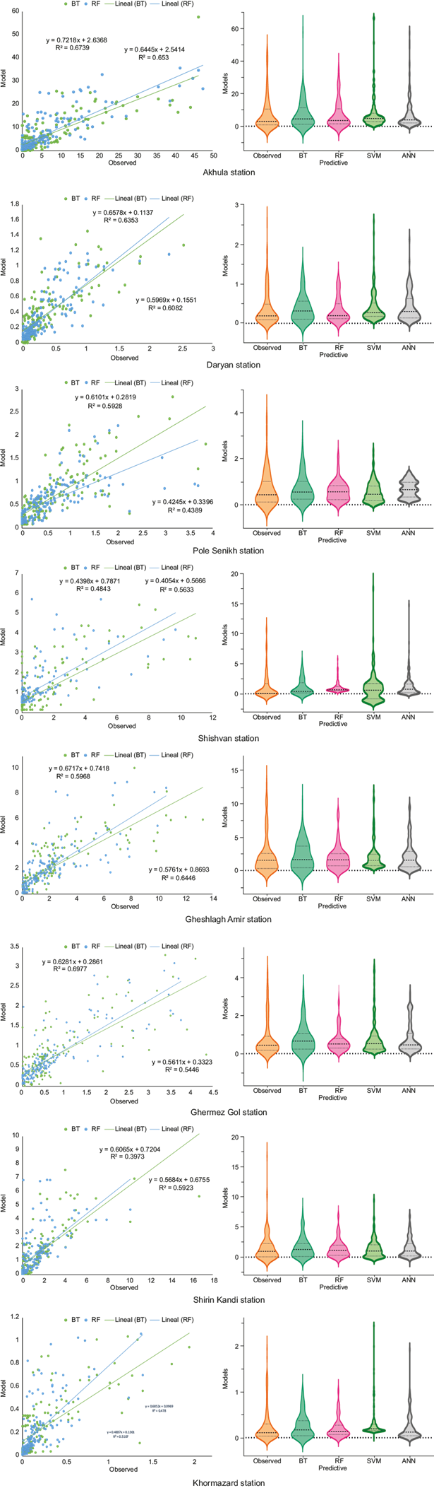
Fig. 7 Verification scatter plots and violin plots of simulated runoff using the Random Forest (RF) and Boosted Tree (BT) models in the eastern sub-basin.
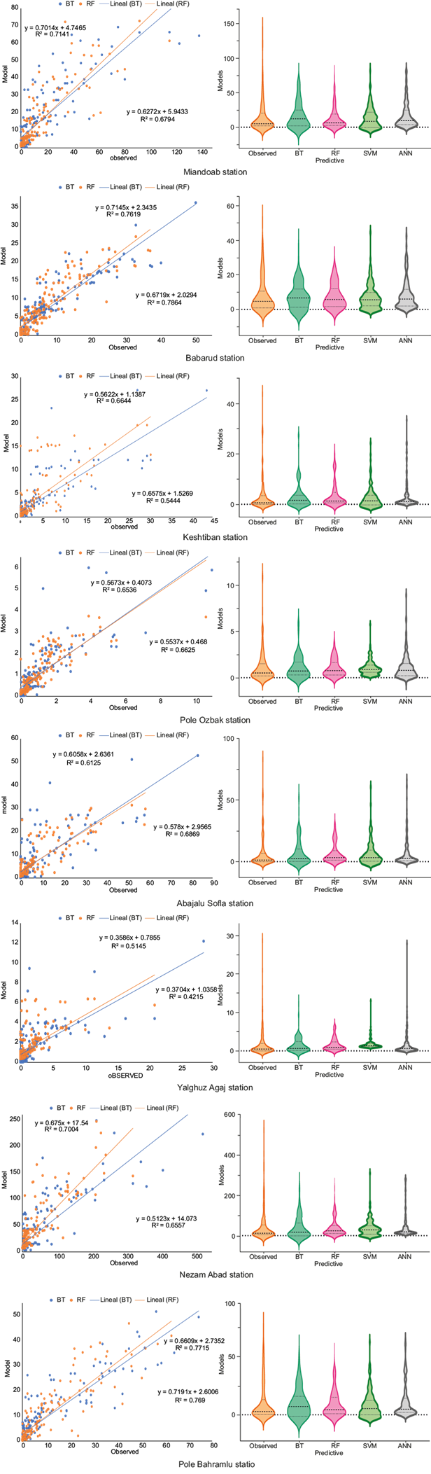
Fig. 8 Verification scatter plots and violin plots of simulated runoff using the Random Forest (RF) and Boosted Tree (BT) models in the western sub-basin.
Similarly, the R2 values for the BT model at Pole Senikh, Shishvan, Gheshlagh Amir, Shirin Kandi and Khormazard stations over the eastern sub-basin were 0.59, 0.56, 0.64, 0.59, and 0.51, respectively, and the R2 values for the western stations Babarud, Keshtiban, and Yalghoz Aghaj were 0.76, 0.82, and 0.51, respectively. Based on the fit line equations and R2 values, it can be concluded that the BT model provides the most accurate estimates for the rainfall-runoff relationship. Also, the linear trends were included to provide a simple, interpretable view of the relationship between observed and predicted values, even if R2 values are less than 0.5. While the models capture non-linear complexities, the linear fits help visualize the overall trend for comparison purposes.
4. Conclusions
This study aimed to enhance rainfall-runoff modeling for 16 key stations in the Urmia Lake basin, Iran. The rainfall and runoff data from 228 rain and 16 runoff gauge stations spanning 43 years (1976-2019) were utilized as hydro-climatic inputs. The objective was to identify the most effective model based on hydrological insights for accurate monthly discharge estimation while considering time lag effects. To achieve this, chronological records of these parameters and regional-scale meteorological inputs were analyzed using heuristic RF and BT methods. Predictor significance for each variable was evaluated, and the RF and BT models were compared. The rainfall-runoff modeling performance of both models for the 16 stations was assessed using training and testing for the whole study period, and the results were compared to determine the best-performing model for each station.
In general, the RF model provided better estimates for the eastern stations Akhula, Daryan, and Ghermez Gol, with CCs of 0.82, 0.80, and 0.84. However, the BT model outperformed RF for the Pole Senikh, Shishvan, Gheshlagh Amir, Shirin Kandi, and Khormazard stations, with CC values of 0.77, 0.75, 0.80, 0.77, and 0.71, respectively. For the western stations, the RF model yielded better estimates for Miandoab, Pole Ozbak, Abajalu Sofla, Nezam Abad, and Pole Bahramlu stations, with CC values of 0.85, 0.81, 0.83, 0.84, and 0.88, respectively. Conversely, the BT model performed better for Babarud, Keshtiban, and Yalghoz Aghaj stations, with CC coefficients of 0.87, 0.82, and 0.72, respectively.
However, the results obtained from these models prove their effectiveness in providing valuable insights for hydrological applications, particularly in rainfall-runoff estimation. A time series analysis of the stations revealed irregular fluctuations in monthly rainfall, with some years showing decreases and others showing increases. Additionally, the runoff trend across the stations indicated a general decrease over time, although some fluctuations were observed. Notably, after 1995, there was a notable increase in the discharge trend. These findings highlight a significant decrease in inflow to Lake Urmia over the past 43 years, with a particularly sharp decline in recent years. This reduction in runoff and inflow can be attributed to several factors, including increased urban water demand and extensive agricultural development, with the agricultural sector being the predominant consumer of water resources from the basin.

