


 nueva página del texto (beta)
 Inglés (pdf)
 Artículo en XML
 Referencias del artículo
 Enviar artículo por email
 Citado por SciELO
  Similares en
SciELO
Similares en
SciELO 
 Permalink
1. Introduction
The COVID-19 pandemic is one of the most severe health crises in recent memory. The official death toll around the world surpassed one million as of September 29, 2020. Considering reporting problems in some countries and that the pandemic is still not under control, the actual death toll may not be known for several years.
Countries worldwide have imposed restrictions on economic activity to slow the rate of infection. Most of the restrictions can be motivated by the early results from the rate of infection in Wuhan, China (Kraemer et al., 2020; Prem et al., 2020). The restrictions on economic activity resulted in mass unemployment and reductions to the GDP worldwide. If the current pandemic follows similar dynamics as previous ones, the economic effects may be felt even in the long run (Rodríguez-Caballero and Vera-Valdés, 2020). In this context, assessing the effect of economic restrictions on public transport mobility and air pollution emissions is of great importance.
Most governments have imposed restrictions on public transport mobility throughout the COVID-19 pandemic. For example, Badr et al. (2020) and Cartenì et al. (2020) document the restrictions in the USA and Italy, respectively. These mobility limits may introduce a structural change in the global dynamic of public transport systems. As in other large cities, the local government in the Mexico City Metropolitan Area (MCMA) has imposed restrictions on the city’s public mobility. The MCMA is an interesting case due to its high population density and the high number of workers in the informal sector. Therefore, it is relevant to formally study whether MCMA’s restrictions cause a statistically significant reduction in passengers in the most used public transport systems: the subway system (Metro) and the bus rapid transit system (Metrobús).
In connection with the study of possible structural changes in public transport mobility, it is crucial to test if the government restrictions also result in lower air pollution levels. The evidence on the effect that restrictions have on pollution levels across the world is mixed. Significant reductions in nitrogen dioxide (NO2) are encountered in, among others, Brazil, India, and Spain (Baldasano, 2020; Shehzad et al., 2020; Nakada and Urban, 2020). However, Adams (2020) finds that PM2.5 (inhalable particles with diameters of 2.5 µm and smaller) levels do not change in response to a region-wide state of emergency in Ontario, Canada. Meanwhile, Berman and Ebisu (2020) find slight declines in PM2.5 levels in the USA, but the results differ significantly between urban and non-urban counties. The authors argue that the different effects of economic restrictions between NO2 and PM2.5 may be explained by the fact that multiple non-transportation sources, including emissions from food industries and biomass burning, contribute to PM2.5 levels. In this regard, they argue for more research on the impacts of the COVID-19 pandemic on industrial sourced pollutants. Moreover, Wang et al. (2020) find that severe air pollution events still occurred in most North China Plain areas even after all avoidable activities in China were prohibited on January 23, 2020.
This paper contributes to the literature by testing the effects of social distancing restrictions on public transport mobility and air pollution in the MCMA. Furthermore, we use the Granger-causality test to show that the precedence relation between public transport mobility and air pollution vanished during the restrictions.
This article proceeds as follows. The following section presents the data used in this study. Section 3 analyzes if the restrictions introduced due to COVID-19 result in structural changes in air pollution levels and mobility in the MCMA, while section 4 presents results from Granger-causality tests between mobility and air pollution in times of COVID-19. Section 5 concludes.
2. Data
The data come from the Portal de Datos Abiertos de la CDMX (Mexico City’s data repository). We gather data on air pollution (PM10, PM2.5, and SO2) levels at all stations and the number of passengers at all Metro and Metrobús stations. The data span from January 1, 2017, to July 31, 2020, and it presents several missing observations and some outliers that we clean first.
Outliers are detected in some of the Metro lines. A few observations (no more than 10 in total) show a thousand-fold increase compared to the rest. We attribute these differences to errors in capturing the data. We remove the outliers and impute them using observations in close proximity. It is worth pointing out that the small proportion of imputed outliers do not qualitatively alter the results.
Missing data are reported for some of the air pollution measuring stations. The missing values seem to randomly occur for some days. To correct the missing values, we use the vast amount of information to construct daily indexes for the air pollution measured in the MCMA. The index construction is motivated by the strong correlation across air pollution measuring stations (Fig. 1). In this regard, missing observations are smoothed out by the construction of the index.
Furthermore, the data show some seasonal patterns.
For the mobility indexes, weekends and holidays show a clear seasonal pattern with a significant decrease in users. We control the seasonality by using data on nearby dates using linear imputation.
For the air pollution indices, the data show some natural seasonal patterns related to the weather. Therefore, we control the seasonality by using monthly dummy variables as is standard in the literature.
3. Structural changes due to COVID-19
The Mexican government established a Jornada Nacional de Sana Distancia (National Campaign of Social Distancing, NCSD), on March 23, 2020 (Secretaría de Salud, 2020). The plan established four measures to mitigate the effects of COVID-19 on the general population: (a) personal hygiene recommendations; (b) suspension of activities deemed non-essential; (c) postponement of mass gathering events (more than 5000 participants); and (c) guidelines for care of the elderly. The plan was heralded by “Susana Distancia”, a fictitious heroine promoting social distancing. The preventive measures ended on May 30, 2020.
The goal of the plan was to impose social distancing measures and slow the spread of the virus. This section uses NCSD as a natural experiment to test if the restrictions introduced structural changes in pollution and public transport mobility.
As a first step, we study the trend mechanism of the series. We employ a broad range of unit root tests: the Augmented Dickey-Fuller (ADF) (Dickey and Fuller, 1979), the Phillips-Perron (PP) (Phillips and Perron, 1988), the Dickey-Fuller Generalized Least Squares (DG-GLS) (Elliott et al., 1996), and the Ng-Perron (Ng and Perron, 1995). In the unit root literature, it is well known that these tests suffer from a loss of power in the presence of structural breaks under the alternative hypothesis. As previously argued, we consider that the restrictions imposed due to COVID-19 provoked an exogenous break as in Perron (1989). Nonetheless, as a robustness exercise, we use unit root tests that allow for endogenous breaks (those not imposed by the practitioner). Therefore, we employ the tests of Zivot and Andrews (1992) (ZA92), that allows for a break under the alternative; Perron (1997), (P97), that allows for structural breaks under both the null and the alternative, and Kapetanios (2005) (K05), which allows for up to three breaks under the alternative.
Table I displays the results from the seven unit-root tests considered. As seen, we reject the null hypothesis of unit root processes in our variables. Note that the ADF and Ng-Perron tests fail to reject the null, possibly due to a loss of power due to the break. Nevertheless, note that the last four tests reject the possible unit root involved. Breaks in ZA92, P97, and K05 tests are located in the neighborhood of March 23, 2020. This date matches the origin of the NCSD.
Table I Unit root tests without constant term for pollutants, Metrobús, and Metro using full-sample data.
| Variable | ADF | PP | DF-GLS | Ng-Perron | ZA92 | P97 | K05 |
| PM10 | -13.31*** | -17.65*** | -4.28*** | -11.07** | -16.72*** | -11.06*** | -14.31*** |
| PM2.5 | -13.70*** | -18.74*** | -2.95*** | -7.84** | -17.30*** | -14.75*** | -14.69*** |
| SO2 | -20.29*** | -23.18*** | -5.05*** | -14.50*** | -21.67*** | -21.46*** | -21.49*** |
| Metrobús | -2.07 | -2.74* | -1.32** | -4.12 | -10.32*** | -9.11*** | -9.09*** |
| Metro | -3.35** | -13.14*** | -3.04*** | -13.33** | -17.50*** | -11.85*** | -14.38*** |
Notes: Lags in ADF and DF-GLS with Schwarz information criteria. Model with constant in PP. Model with intercept in ZA92 with two lags. P97 test considering model A. *, **, and *** denote rejection of the null hypothesis (unit root) at 10, 5, and 1%, respectively.
Moreover, given that aggregation is used to construct the indexes, we estimate the fractional difference parameter for the series (Granger, 1980; Haldrup and Vera-Valdés, 2017). We use semiparametric estimators in the frequency domain to avoid the effect of the mean’s specification to affect the results (Geweke and Porter-Hudak, 1983; Künsch, 1987; Shimotsu and Phillips, 2005). Results from the long memory estimates are presented in Table II. All tests find the data to be in the stationary range, well below the unit root scenario. Note that all stationarity tests consider the subperiod between January 1, 2017, and December 31, 2019, to avoid spurious results due to the possible structural change (Martínez-Rivera et al., 2012).
Table II Long memory estimates, confidence intervals are shown below. Standard T1/2 bandwidth where T is the sample size.
| Variable | GPH | LW | ELW |
| Metro | 0.199 | 0.234 | 0.271 |
| [-0.021-0.419] | [0.063-0.405] | [0.100-0.442] | |
| Metrobús | 0.643 | 0.632 | 0.660 |
| [0.423-0.863] | [0.461-0.803] | [0.483-0.831] | |
| PM10 | 0.408 | 0.378 | 0.419 |
| [0.188-0.628] | [0.207-0.549] | [0.248-0.590] | |
| PM2.5 | 0.347 | 0.358 | 0.402 |
| [0.127-0.567] | [0.187-0.529] | [0.231-0.573] | |
| SO2 | 0.184 | 0.174 | 0.201 |
| [-0.036-0.404] | [0.003-0.345] | [0.030-0.372] |
GPH: Geweke and Porter-Hudak (1983) long memory estimators; LW: Künsch (1987) long memory estimators; ELW: Shimotsu and Phillips (2005) long memory estimators.(1983)
Once we guarantee that our data is stationary, we consider the following specification to test for a structural change:
where y t is the air pollution or mobility measure, and t = [1,2,…,T]', with T the sample size. Furthermore, DU and DT are dummy variables that model the possible structural change due to NCSD. That is, DU = [0,…,0,1,…,1]', and DT = [0,…,0,1,2,…,T 1 ]', where the non-zero elements start on March 23, 2020, and T 1 is the size of the subsample after that date. We test for a change in level if α 1 ≠ 0, and for a change in both level and trend if α 1 ≠ 0 and β 1 ≠ 0.
The test for structural change proceeds as follows:
Estimate the unrestricted model (Eq. [1]), and recover the unrestricted residual sum of squares, URSS, given by URSS = Σe t 2 , where e t are the residuals from estimating Eq. (1).
Estimate the restricted model (Eq. [1]), with α 1 = 0 and β 1 = 0, or β 1 = 0, and recover the restricted residual sum of squares, RRSS. The restricted sum of squares is given by URSS = Σe t 2 , where e t are the residuals from estimating Eq. (1) imposing α 1 = 0 and β 1 = 0, or β 1 = 0.
-
where T is the sample size, k is the number of parameters in the unrestricted model, and r is the number of restrictions.
The test statistic follows an F distribution with r and T - k degrees of freedom.
The structural change test assumes that the date of the break is known. As argued above, the restrictions due to COVID-19 are considered exogenous with a precise start date. Thus, the assumptions of the F-test are satisfied. Nonetheless, as a robustness exercise, we use the method developed by Bai and Perron (1998) to estimate the date of the break endogenously.
3.1 Mobility data
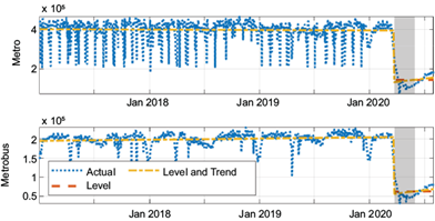
Figure 2 presents the mobility indexes for Metro and Metrobús. The data range from January 1, 2017, to July 31, 2020. The shaded region contains the period considered in NCSD. Also plotted are the estimates from the linear model in Eq. (1). We allow for both a change in level and a change in level and trend at the start of the NCSD. As can be seen from the figure, the dynamics of the mobility indices change significantly due to NCSD.
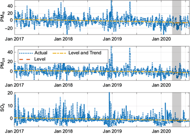
Fig. 2 Mobility indices in the Mexico City Metropolitan Area. The figure shows actual values (dotted blue) along with fitted values from the linear models with a change in level (dashed orange) and change in level and trend (dashed-dotted yellow). NCSD is shown in the shaded area.
Table III presents the estimates from Eq. (1) allowing for a change in level and a change in level and trend and the structural change test results. The table presents some interesting findings. First, note the different results regarding the trend coefficient, β 0 . There is no significant trend in the number of Metro users, while a significant but small positive trend in Metrobús users over the last three years. The results suggest that more people started using public transit systems in the MCMA in the last few years.
Table III Unrestricted equation estimation and test for structural change.
| Variable | Change in level | Change in level and trend | |||||||
| α 0 | β 0 | α 1 | F | α 0 | β 0 | α 1 | β 1 | F | |
| Metro | 4(105)*** | -5.386 | -3(105)*** | 2086*** | 4(105)*** | -5.682 | -3(105)*** | 215* | 1046*** |
| Metrobús | 2(105)*** | 42.5*** | -2(105)*** | 7006*** | 2(105)*** | 42.4*** | -2(105)*** | 69.3* | 3510*** |
| PM10 | 4.412*** | -0.01*** | -1.322 | 1.101 | 4.428*** | -0.01*** | -2.681 | 0.021 | 0.849 |
| PM2.5 | 1.806*** | -0.00*** | -1.431* | 3.149* | 1.805*** | -0.00*** | -1.384 | -0.001 | 1.574 |
| SO2 | 1.027*** | -0.00*** | -0.028 | 0.006 | 1.029*** | -0.00*** | -0.157 | 0.002 | 0.039 |
*, **, and *** denote rejection of the null hypothesis at 10, 5, and 1%, respectively.
Second, note the statistically significant decrease in the level of public transport users associated with NCSD. These results are in line with those from Badr et al. (2020) and Cartenì et al. (2020) for the USA and Italy. For the MCMA, the structural change is quite significant. The number of users more than halved during NCSD. That is, most users seem to have followed the government’s recommendations and avoided the public transport system. Nonetheless, given the lack of data on the number of private cars and their number of passengers, we cannot extrapolate this result to state that people remained at home during NCSD. Furthermore, as a robustness exercise, we test all Metro and Metrobús lines individually for a structural change (Table IV and Fig. 3). The results from the robustness exercise are in line with the ones for the indices.
Table IV Structural change test for individual Metro and Metrobús lines and number of cyclists at several reporting stations.
| Mobility | F level | F trend |
| Metro Line 1 | 1839*** | 930*** |
| Metro Line 2 | 1729*** | 865*** |
| Metro Line 3 | 1030*** | 515*** |
| Metro Line 4 | 1382*** | 691*** |
| Metro Line 5 | 934*** | 467*** |
| Metro Line 6 | 945*** | 471*** |
| Metro Line 7 | 953*** | 476*** |
| Metro Line 8 | 1523*** | 762*** |
| Metro Line 9 | 760*** | 380*** |
| Metro Line A | 559*** | 280*** |
| Metro Line B | 1878*** | 943*** |
| Metro Line 12 | 1134*** | 533*** |
| Metrobús Line 1 | 5429*** | 2716*** |
| Metrobús Line 2 | 2947*** | 1471*** |
| Metrobús Line 3 | 5646*** | 2824*** |
| Metrobús Line 4 | 4993*** | 2616*** |
| Metrobús Line 5 | 4469*** | 2232*** |
| Metrobús Line 6 | 3446*** | 1720*** |
*, **, and *** denote rejection of the null (no structural change) at 10, 5, and 1%, respectively.
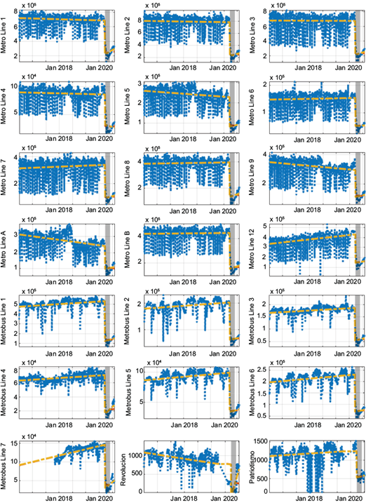
Fig. 3 Mobility in the MCMA. The figure shows actual values (dotted blue) along with fitted values from the linear model with a change in level (dashed orange) and change in level and trend (dashed-dotted yellow). NCSD is shown in the shaded area.
Regarding the method to estimate the break endogenously, it finds the break date on March 21, 2020, with NCSD contained in the confidence interval. That is, the date of the break estimated endogenously coincides with the start of NCSD.
3.2 Pollution data
Figure 4 presents the air pollution indices. The figure shows PM10, PM2.5, and SO2 levels from January 1, 2017, to July 31, 2020. The shaded region contains the period considered in NCSD. Also plotted are the estimates from the linear model in Eq. (1). We allow for both a change in level and a change in level and trend at the start of the NCSD. As shown in the figure, the dynamics of air pollution do not significantly change due to NCSD.
Fig. 4 Pollution indices in the Mexico City Metropolitan Area. The figure shows actual values (dotted blue) along with fitted values from the linear model with a change in level (dashed orange) and change in level and trend (dashed-dotted yellow). NCSD is shown in the shaded area.
Furthermore, Table III presents the estimates from Eq. (1) allowing for a change in level and a change in level and trend and the structural change test results. The table presents some interesting findings.
First, the estimates show a significant decreasing trend for all pollutants across the period considered. Nonetheless, the estimates from the trend parameter are relatively small. Air pollutant levels have been decreasing through the years, but the decrease seems to be occurring at a slow pace.
Second, note that the null of no structural change is not rejected for both tests. The restrictions imposed by NCSD do not seem to be associated with a lower level of air pollution. These results are in line with the ones reported by Adams (2020) for Ontario, Canada. The author finds no significant reduction in PM2.5 resulting from restrictions imposed due to COVID-19. Moreover, Wang et al. (2020) find that severe air pollution events still occurred in most of the North China Plain areas, even after all avoidable activities in China were prohibited on January 23, 2020.
Third, NCSD can be considered a natural experiment regarding public transport usage on air pollution. The lack of structural change in air pollution during NCSD coupled with the significant decrease in the mobility indices point to a non-significant effect of the number of users of the public transport system on pollution. As argued before, this may relate to a higher number of private cars during NCSD. Thus, these results suggest that tackling air pollution in the MCMA requires specific policies to reduce private car usage, particularly in light of the positive willingness to pay for clean air by inhabitants of the MCMA (Rodríguez-Sánchez, 2014; Filippini and Martínez-Cruz, 2016; Fontenla et al., 2019).
Finally, regarding the method to estimate the date of the break endogenously, the method does not find a break in 2020. Thus, our results are robust to an endogenous specification of the date of the break.
To properly assess the relationship between public transport and air pollution, the following section uses the Granger-causality test to assess if there exists a relation of precedence between them. Furthermore, we test if there is a change in this relationship after NCSD.
4. Granger-causality
In this section, we test the type of relation that exists between public transport mobility and air pollution indices. We use the concept of causality developed by Granger (1969). Although sometimes misrepresented in the literature, the test evaluates if a variable x has explanatory power on the variable y in the sense that x precedes y. We interpret this precedence as changes in variable x being related to changes in variable y. Note that this does not necessarily denote a causal relation, given that a third variable could be driving both x and y. Nonetheless, the literature has settled on denoting this type of test as Granger-causality tests.
The test for Granger causality proceeds as follows:
-
where k, m are the number of lags included in the regression. In applied work, k = m is common. From the estimation, we recover the residual sum of squares, URSS. Our analysis considers specifications with the same number of lags for both variables from the previous day and two days before.
-
and recover the residual sum of squares, .
-
where T is the sample size, k is the number of parameters in the unrestricted model, and m is the number of restrictions.
The test statistic follows an F distribution with m and T - k - m - 1 degrees of freedom.
Intuitively, the test for Granger-causality assesses if the extra information contained in the additional variable helps explain the dynamics of the dependent variable better than the information contained in the lags of the dependent variable alone. This additional explanatory power is denoted in the literature as a precedence relation.
Granger-causality has been shown to produce spurious results (rejection of the null when the null is true) when the data follow processes with structural breaks or unit root processes (Ventosa-Santaulària and Vera-Valdés, 2008; Rodríguez-Caballero and Ventosa-Santaulària, 2014). Thus, our methodology relies on testing for Granger-causality before NCSD and contrast the results against estimation in the period after NCSD to avoid spurious results.
Table V presents the results from the Granger-causality test for the period before NCSD. The table shows that Metrobús Granger-causes air pollution in terms of PM10 and SO2. Thus, there is statistical evidence that Metrobús usage changes are associated with PM10 and SO2 air pollution changes. Nonetheless, recall that we cannot conclude that changes in Metrobús usage cause changes in air pollution in the typical sense, given that a third common factor for both could be the main driver behind both dynamics. In this context, more Metrobús users could be associated with more economic activity and more cars on the road.
Table V Test for public transport Granger-causing air pollution in the periods before and after NCSD. The tests consider specifications including lags from the previous day, GC(1), and two days before, GC(2).
| Variable-period | PM10 | PM2.5 | SO2 | |||
| GC(1) | GC(2) | GC(1) | GC(2) | GC(1) | GC(2) | |
| Metro pre-NCSD | 0.269 | 0.169 | 0.170 | 0.201 | 0.873 | 0.691 |
| Metro post-NCSD | 1.315 | 1.470 | 0.680 | 0.506 | 2.170 | 0.667 |
| Metrobús pre-NCSD | 3.448* | 3.324** | 0.477 | 0.915 | 4.090** | 2.860* |
| Metrobús post-NCSD | 1.829 | 1.816 | 0.803 | 0.536 | 2.602 | 0.867 |
*, **, and *** denote rejection of the null hypothesis (no Granger-causality) at 10, 5, and 1%, respectively.
To evaluate the effect that NCSD had on the precedence relation between public transport mobility and air pollution, Table V presents the results from the Granger-causality test for the post-NCSD period. The table shows that Granger-causality between public transport mobility variables and PM10 and SO2 disappeared during NCSD. That is, changes in mobility indices do not precede changes in air pollution indices. In this regard, we argue that other sources of air pollution like industry and private car usage may be the major contributors to air pollution in the MCMA.
Overall, the results from the Granger-causality analysis support the notion that the link between public transport users and air pollution was temporarily broken during NCSD. The reduction in public transport users during NCSD was not accompanied by a reduction in air pollution.
5. Conclusions
This paper analyzes the relation between COVID-19, air pollution exposure, and mobility in the MCMA.
We test if the Mexican Government’s economic and social restrictions to mitigate the spread of the virus produced a structural change in air pollution and mobility in the MCMA. Our results show that mobility in public transportation was significantly reduced following the government’s recommendations. We find that mobility in public transit systems in the MCMA decreased by more than 65%. Thus, our results suggest that a large share of the inhabitants of the MCMA stopped using public transit during this period.
In connection with the structural change in mobility, we analyze if the restrictions resulted in lower air pollution in the MCMA. Our results show an overall decreasing trend in pollution levels in the MCMA throughout the years. Nonetheless, no statistically significant change is detected as a result of economic restrictions imposed due to COVID-19. That is, air pollution levels and trends were not affected as a product of the economic restrictions.
Furthermore, we use the Granger-causality test to analyze the existence of a precedence relation between public transport users and air pollution. Our results show that before the emergence of COVID-19, changes in public transport users were associated with changes in air pollution. Nonetheless, the precedence relation between public transport mobility and air pollution disappeared following the restrictions. These results suggest that additional factors as private car usage or industrial pollution may be more significant factors behind changes in air pollution.
The results from this analysis could help in designing policies aimed to reduce pollution levels in the MCMA. Structural changes in mobility in the public system do not seem to be associated with changes in air pollution levels. In this regard, our results suggest that tackling air pollution requires policies aimed explicitly at reducing industrial pollution and private car usage.

