


 nueva página del texto (beta)
 Inglés (pdf)
 Artículo en XML
 Referencias del artículo
 Enviar artículo por email
 Citado por SciELO
  Similares en
SciELO
Similares en
SciELO 
 Permalink
1. Introduction
Between February and March of 2017, extreme precipitation was registered along the north and central coast and highlands of Peru, reaching values over 120 mm/day in north coastal cities, where the monthly average is 28 mm (Figs. 1 and 2), associated with an abnormal warming of the sea surface temperature (SST) above 28 ºC (Garreaud, 2018) in El Niño 1+2 region, mainly during March.
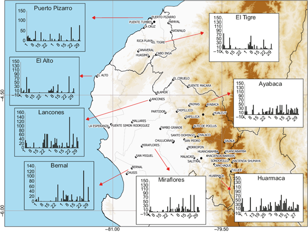
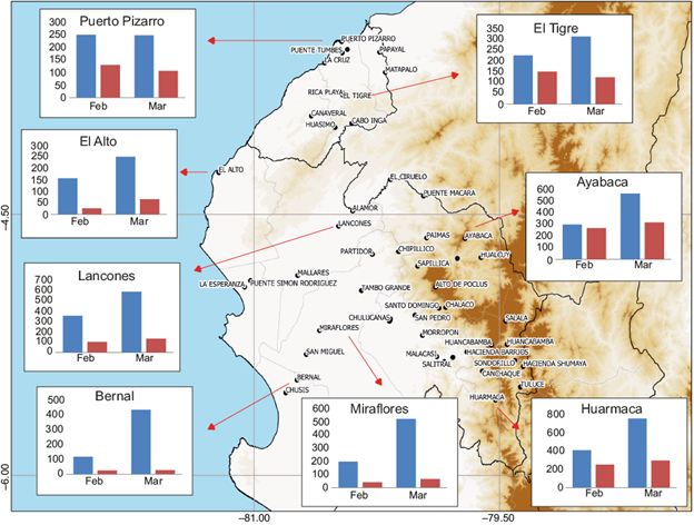
Fig. 2 Monthly precipitation during February and March, 2017 in Tumbes and Piura (2017 monthly accumulated: blue; normal monthly accumulated: red).
According to Rodríguez-Morata et al. (2018), the rainfall recorded between January and March 2017 can only be compared with the extreme El Niño events of the last 40 years, and exceeded the 90th percentile (1981-2017), causing floods and landslides (locally known as huaicos) in the arid coast zone. These hydrometeorological events were caused by an unusual type of El Niño, the coastal El Niño (Takahashi and Martínez, 2017; Takahashi et al., 2018).
According to Ramírez and Briones (2017), economic losses due to coastal El Niño-related precipitation were estimated at USD 3.1 billion and affected over 1 million people (INDECI, 2017), with at least 113 killed and nearly 40 000 homes destroyed (Fraser, 2017). The most affected Peruvian regions were Piura, Lambayeque, La Libertad and Lima. An array of infectious diseases, like dengue, chikungunya, zika and leptospirosis, also were reported (Ramírez and Briones, 2017), triggered by stagnant water, increased humidity and warm air temperatures observed during this period (1-2.5 ºC above its normal between January and March) (ENFEN, 2017a, b).
2. The 2017 coastal El Niño (CEN)
Echevin et al. (2018) did a complete analysis of the 2017 CEN and concluded that the initial warming was mainly associated with a regional decrease of winds in the far-eastern Pacific from late 2016 to January 2017. This wind relaxation reduced the coastal upwelling and vertical mixing in the top ocean layers, generating a positive SST anomaly off northern Peru and Ecuador, which resulted on an alongshore temperature gradient.
During February and March (FM), the Ekman pumping negative anomaly may have deepened the thermocline, generating anomalously warm source waters. Peng et al. (2019) concluded that both the downwelling oceanic Kelvin waves, observed in December 2016 (ENFEN, 2017a), and local northerly alongshore wind anomalies were necessary for an extreme CEN. The latter caused the average magnitude of the southeast trade winds in the austral summer of 2017 to be one of the lowest in the 1948-2016 period, favored by anomalous easterly winds in the mid- and upper troposphere, which did not contribute to the tropospheric sinking and strengthening of the trade winds (Garreaud, 2018). According to Hu et al. (2019)), the formation of the 2017 CEN was largely driven by ocean heat flux anomalies, associated with westerly surface wind anomalies in the equatorial far-eastern Pacific, mainly during January, the biggest for that month since 1981 (Takahashi et al., 2018).
Although coastal El Niño and basin-scale El Niño occur simultaneously most of the time, so that Niño 3.4 and Niño 1+2 indices are positively correlated (Hu et al., 2019), FM Peruvian coastal warming is not always preceded by a basin-scale Niño. In fact, the strong event of 2017 was preceded by a weak basin-scale La Niña (Xie et al., 2018; Peng et al., 2019).
The first CEN analyzes were done by Takahashi and Martínez (2017), focused on the events of 1891 and 1925. These CEN were generated by strong northerly winds across the equator in the equatorial eastern Pacific and the strengthening of the Intertropical Convergence Zone (ITCZ) south of the equator.
Hu et al. (2019) identified seven CEN between 1979 and 2017, which were driven by three different mechanisms. The CEN of 1983, 1987 and 1998, as they occurred immediately after extreme/strong El Niño, were driven by an equatorially centered ITCZ that generated anomalously strong convection in the eastern tropical Pacific, leading to the relaxation of the southeast trade winds suppressing the wind-forced upwelling and resulting in warming in the eastern tropical Pacific. The CEN of 2014 and 2015 were associated with thermocline fluctuations driven by eastward propagation of a downwelling Kelvin wave, warming the eastern tropical Pacific. Lastly, the CEN of 2008 and 2017 were associated with westerly surface wind anomalies in the eastern equatorial Pacific and largely driven by ocean surface heat flux. As far as the frequency of extreme CEN, there is an increase in a warming climate (Peng et al., 2019).
One of the main factors that favored the extreme rain in the CEN was related to the development of the second band (south band) of the eastern Pacific ITCZ. Here, we show a detailed analysis of the behavior of this band during early 2017, associated with a synoptic circulation and energetic analysis. A description of the ITCZ second band is detailed in section 2, followed by a description of the data and methodology used in this research (section 3). In section 4 the results are shown and discussed. Finally, in part V the conclusions of this study are presented.
3. The ITCZ second band
The interannual variability of eastern Pacific convection during February-March-April (FMA) has two modes. One with intensified deep convection centered on the equator (single ITCZ), and one with a meridional dipole with little signals on the equator (double ITCZ) (Xie et al., 2018; Yu and Zhang, 2018), due to a cold tongue or lower SST present between the two bands of the ITCZ (Zhang, 2001; Gu et al., 2005). In the latter, there are maximum precipitation anomalies to either side of the equator. These two ITCZ bands develop early during the austral autumn (March-April) in the eastern Pacific (90º-130º W), which coincides with the maximum SST in the equator and south of it, and with the seasonal weakening of southeasterly trade winds (Gu et al., 2005). Likewise, during El Niño events, the ITCZ bands vary according to the ENSO pattern present over the eastern Pacific; an extreme El Niño pattern has a strong ITCZ presence over the equator, while a moderate El Niño pattern presents an ITCZ north to the Equator (Peng et al., 2020).
Haffke et al. (2016) carried out a daily analysis of the ITCZ in the eastern Pacific with satellite information, using an identification method proposed by Henke et al. (2012), and found five states of the ITCZ: the double ITCZ state (dITCZ), where an ITCZ is visible on both sides of the equator; the northern state (nITCZ), and the southern state (sITCZ), where only one ITCZ is formed accordingly; the state of non-presence (aITCZ), where there is no significant ITCZ signal; and the equatorial state (eITCZ), where convection in the eastern Pacific is located on the equator and covers a broad north-south band. The sITCZ state can be viewed as an extreme case of the dITCZ state. The ocean-atmosphere interaction in the Central Pacific (CP) La Niña conditions favor the dITCZ and sITCZ states, with higher correlation in the last one (Yang and Magnusdottir (2016); Yu and Zhang (2018).
From 2000 to 2017 there was an increase of the sITCZ (ITCZ second band) formation (Son et al., 2019); hence, its analysis and relationship with the precipitation in the northern coast of Peru is important.
4. Data and methodology
4.1 ITCZ identification Index
Yu and Zhang (2018) proposed an index to identify the ITCZ second band formation, working with monthly precipitation averaged in three areas (Fig. 3), the northeastern equatorial Pacific (NEP; 180º-85º W, 2º-10º N), the southeastern equatorial Pacific (SEP; 150º-85º W, 10º-2º S), and the eastern equatorial Pacific (EEP; 180º-85º W, 2º S-2º N). In this work, these areas are used to calculate the Yu and Zhang index with monthly and daily satellite estimated precipitation data; also, a new area to identify the formation of the ITCZ second band near the Peruvian coast is proposed. The longitudinal limits of this new area are 91.5º-81.5º W (purple area in Fig. 3), and the same latitudinal limits of NEP, SEP and EEP.
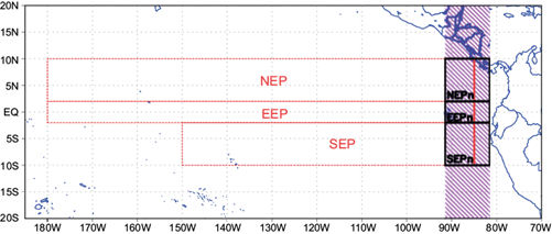
Fig. 3 Areas taken into account for analyzing the ITCZ second band. Yu and Zhang areas (red boxes): NEP (180º-85º W, 2º-10º N), EEP (180º-85º W, 2º S-2º N), SEP (150º-85º W, 10º-2º S). New areas (black boxes): NEPn (91.5º-81.5º W, 2º-10º N), EEPn (91.5º-81.5º W, 2º S-2º N), SEPn (91.5º-81.5º W, 10º-2º S). Purple region is the area considered for temporal wind and precipitation analysis (Fig. 5).
To show the behavior of the early 2017 rain in the Peruvian western north, we selected eight stations of the National Service of Meteorology and Hydrology (SENAMHI) network distributed in Tumbes and Piura (Figs. 1 and 2).
Daily and monthly estimated precipitation from of TRMM Multi-Satellite Precipitation Analysis (TMPA) January 1 to April 30, with 0.25º of spatial resolution, were used in this work (Huffman and Bolvin, 2017),
For SST and its anomalies (SSTA), data of the Operational Sea Surface Temperature and Sea Ice Analysis (OSTIA) reanalysis was used with a spatial resolution of 0.25º and 1-day temporal resolution (Donlon et al., 2012).
Data from the Era-Interim reanalysis (Dee et al., 2011) was also used with a spatial resolution of 79 km (~0.75º), a temporal resolution of 6 h and 37 pressure levels (from 1000 to 10 hPa). The data used is of 12:00 UTC from January 1 to April 30 2017, while the 1981-2010 period was used for the climatology, as recommended by WMO (2014).
For the synoptic analysis, 5-day anomalies of surface winds, sea level pressure, 600 hPa mixing ratio and 200 hPa divergence and winds were considered.
The ITCZ could be identified with analyzes of cloud, precipitation or surface winds (Haffke et al., 2016), and precipitation estimated by TMPA-TRMM, which was used in this paper.
To determine the formation of the ITCZ second band, two indices proposed by Yu and Zhang (2018) to characterize interannual variability of the eastern Pacific ITCZ during boreal spring (February to April) were used: the asymmetric index (Ia) and double ITCZ index (Id):
where P NEP is the boreal spring precipitation rate averaged in the NEP, P SEP is the precipitation averaged in the SEP, P EEP is the precipitation averaged in EEP, and P m is the mean precipitation rate in the three regions:
A negative Id index indicates single precipitation maximum at the equator, while positive a Id index indicates double ITCZ. The Ia index distinguishes the preference of the ITCZ to the north (Ia > 0) or south (Ia < 0) of the equator, or a symmetric double ITCZ (Ia = 0).
Using these indices with precipitation between 1979 and 2017, Yu and Zhang (2018) identified 13 years with maximum precipitation anomalies to the south of the equator: 1984, 1986, 1989, 1996, 1999, 2000, 2001, 2006, 2008, 2009, 2011, 2012, and 2017.
4.2. Lorenz Energy Cycle
The general circulation of the atmosphere may be approximated as a composition of the mean zonal motion and eddies superposed upon it. This allows the division of kinetic (K) and available potential (A) energy of the atmosphere in two types: zonal (Z) and eddy (E). The zonal component of energy surges due to variance of zonally averaged temperature, while the eddy component of energy is associated with the variance of temperature within the latitude circles. Each type of energy is a source or sink of another type (Lorenz, 1955).
Applying the equations of continuity, thermodynamic and motion, and considering transfer of energy across the boundaries in a limited area, Michaelides (1987) proposed the next equations to express the local variation of A Z , A E , K Z and K E as:
where Z and E represent zonal and eddy energies, respectively.
According to Lorenz (1967), A Z represents the amount of available potential energy that would exist if the mass field was replaced by its zonal average, and A E the excess of available potential energy over A Z . Likewise, K Z represents the amount of kinetic energy which would exist if the existing zonally averaged motion, but no eddy motion was present, and K E , the excess of kinetic energy over K Z .
In Eqs. (4-7), G Z represents the generation of zonal available potential energy (A Z ) through the latitudinal differential heating, produced by the diabatic heat sources (Asnani, 1993, 2005). G E represents the generation of eddy potential energy (A E ) along the same latitude, heating the warm regions and cooling the cold regions, generating gradients of temperature in the same latitude. Physically, the latent heat released due to convection should be an important source of heat and, and consequently of eddy available potential energy (G E ) (Dias, 2010). C A (A Z , A E ) represents the conversion of the available potential energy between zonal and eddy forms, associated with meridional and vertical gradients of temperature, transporting sensible heat. In physical terms, the zonal averaged temperature in the troposphere decreases toward the poles, and this gradient generates transport of warm tropical air to polar latitudes and cold polar air to warm latitudes through meridional motions. This process decreases the thermal gradient between latitudes, diminishing A Z , and increases the thermal gradient at the same latitude, resulting in A E increases, related to wave motion (troughs and ridges) and it is an intermediate process in the baroclinic chain. C Z (K Z , A Z ) indicates the conversion of zonal kinetic energy (K Z ) into zonal available potential (A Z ) through upward movements of warm air in low latitudes and downward movements of cold air in high latitudes. According to Asnani (2005), the Hadley and Ferrel circulations are manifestations of this conversion. Meanwhile, C E (A E , K E ) represents the conversion of eddy available potential (A E ) into eddy kinetic energy (K E ) through upward motions of warm air and downward movements of cold air along the same latitude circle. The equatorial Walker circulation would be a manifestation of this process (Aliaga, 2017). C K (K E , K Z ) represents the conversion of the kinetic energy between eddy and zonal types. According to Lorenz (1967), there is no process that converts A Z into K E or A E into K K . D K and D E represent the effects of friction (dissipation) by zonal and eddy motions, respectively. Terms with B represent energy flux across the boundary. All these terms can be expressed in the diagram in Figure 4.
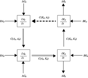
Fig. 4 Diagram of the Lorenz energy cycle (LEC) in a limited area (Michaelides, 1987). Arrows denote the most likely direction of the conversion between energy components for a large-scale mid-latitude region averaged over the passage of many disturbances.
In terms of physical processes in the atmosphere, C K (K K , A K ) and C E (A E , K E ) are denominated baroclinic terms because they are strongly related to the processes that presents baroclinic instability (Dias, 2010) or thermal gradients. On the other hand, C K (K E , K Z ) is called barotropic term (Asnani, 1993, 2005; Dias, 2010).
Studies of the energetics of synoptic systems using Lorenz cycle in a limited area (considering the transfer of energy across boundaries) proposed by Muench (1965) were performed by different authors such as Brennan and Vincent (1980), Michaelides (1987), and Dias and Da Rocha (2011) while researching cyclones; Veiga et al. (2013) used it to study the Walker circulation and its relationship with ENSO; Norquist et al. (1977) and Hsieh and Cook (2007) to evaluate African easterly waves; Da Silva and Satyamurty (2013) in the ITCZ in the South American sector of the Atlantic Ocean; Ramírez et al. (2009) in a work about the energy of the South American rainy season.
Here, the daily temporal variation of integrated energy components in the atmospheric volume in the ITCZ second band near the Peruvian coast was studied, using the LEC in a new SEP area (SEPn) (from -10º to -2º S and from 91.5º to 81.5º W) (Fig. 3) from January 1 to April 30, 2017.
5. Results
5.1. Temporal variability of the ITCZ’s second band near the coast
The temporal variability of precipitation, SST, and 10 m wind, as well as its anomalies, averaged between 91.5º and 81.5º W in early 2017 (Fig. 4) shows the presence of the ITCZ second band between the end of January and the beginning of April. The highest intensity of the second band occurred during February and March. The south trade wind relaxation reported by Garreaud (2018) and Hu et al. (2019), even with anomalies from the north, is observed during January, February and March, mainly between 5º N and 10º S, and in April returned to its normality (Fig. 4b).
There were two defined periods with formation of the ITCZ second band, determined only by precipitation anomalies: one from the last days of January to the first half of February, and another during March (purple boxes in Fig. 4b). These periods were preceded by an anomalously warm SST since the beginning of January, and by anomalous winds from the north 10 days before (Fig. 4b). It is possible that the relaxation of the southeast trade winds is associated with the behavior of the South Pacific Anticyclone.
Fig. 4b shows that the surface winds were anomalously from the north between January and March, with two main episodes: the second half of January and March, in the 5º N to 10º S strip. This is similar to Echevin et al. (2018), who found that the anomalies of wind stress nearshore and offshore in January 2017 were poleward.
It is observed that the nuclei of maximum precipitation in the ITCZ second band are toward the south of the SST maximum. This is consistent with Gu et al. (2005), who found that the precipitation maximum is out of phase toward the poles of the SST maxima.
SST exceeding the threshold of 27 ºC is one of the main factors that favor the development of the ITCZ second band near the coast (mainly when this value is above its normal by 2º C during FM, at least). This threshold is not necessarily required to maintain the first band (Fig. 4). However, a warming of the SST is not sufficient to generate precipitation alone, the behavior of the wind is also important. According to Yu and Zhang (2018) in the SEP there is no significant relationship between the local SST and precipitation, as there is in the NEP.
In early January, an anomalous westerly wind over the equatorial Pacific was observed, which preceded the formation of the ITCZ second band near the coast between January 31 and February 4, 2017 (Fig. 5). This is congruent with Peng et al. (2019)), who manifested that these strong westerly winds, which were the largest for January since 1981 (Takahashi et al., 2018), together with anomalous northerly coastal winds, caused the downwelling Kelvin waves, also found by ENFEN (2017a).
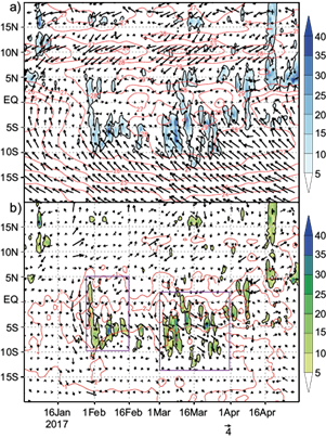
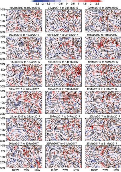
Fig. 5 (a) Daily SST (ºC, contours), daily precipitation (mm day-1, shaded) and 10 m wind (m s-1, vectors). (b) Daily SST anomalies (ºC, contours), daily precipitation anomalies (mm day-1, shaded) and 10 m wind anomalies (m s-1, vectors). The values are averaged between 91.5º and 81.5º W. Purple boxes represent the ITCZ second band events.
Between January 21 and 25 the northerly anomalies in the wind were most prevalent in the analysis region. In the period between February 10-14, the highest intensity of westerly anomalously winds over 110º-90º W was observed, while March was characterized by westerly and northerly anomalous winds (Fig. 5). It is also clear that in the second half of February there was an absence of rainfall in the region.
5.2. Atmospheric circulation
In Fig. 6 we can see that, between January and the first 10 days of February, the MSLP was below its normal in the east of the South Pacific, contrasting with the positive anomaly of MSLP in the equator from 100º W to the west. This contrast of pressure can be associated with the intensification of westerly and northerly winds in the equator close to the Peruvian coast (Fig. 7). This is congruent with Takahashi (2004), who suggested that rainy days during 1997-1998 and 2002 El Niño events were associated with an enhanced onshore westerly low-level flow, which may help the triggering of convection by orographic lifting over the western slope of the Andes.
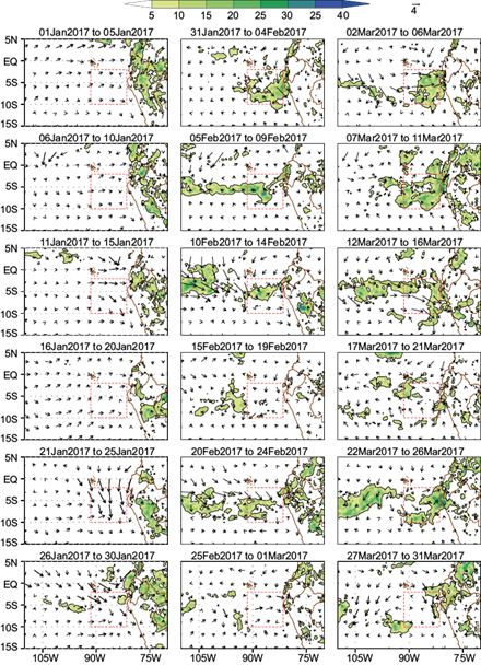
Fig. 6 Five-days mean sea level pressure (hPa, contours) and sea surface temperature (ºC, shaded) anomalies.
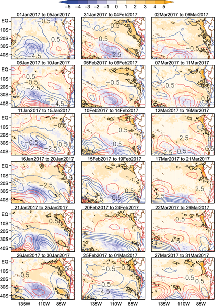
Fig. 7 Five-days precipitation (mm day-1, shaded) and 10 m wind (m s-1, vectors) anomalies. Red boxes represent the new SEP area (SEPn).
After that and until February 24, the MSLP was above its normal in the Southeast Pacific, causing a decrease of rainfall in the second half of February (Fig. 5). Then, between the last days of February and the first half of March, the negative MSLP anomaly in the east of the South Pacific returned, favoring a new increase in rainfall close to the equator, near and over the Peruvian coast. During this period, the MJO was more active and influenced the intensification of surface westerlies in the oriental Pacific near the Equator, as explained in Tang and Yu (2008).
The positive SST anomaly near the Peruvian coast was increasing in intensity and area since January 16, which favored the convection producing low-level convergence of the thermally driven boundary layer winds (Lindzen and Nigam, 1987 apud Takahashi, 2004).
In 600 hPa (Fig. 8), the positive anomalies of mixing ratio (MIXR) in the region of the ITCZ second band near the coast developed around January 21-25, with highest intensity between January 31 and February 4 and positive MIXR flux from east to west. From February 10 to March 1, negative anomalies of MIXR in the region of the ITCZ second band can be observed near the coast, associated with the decrease of rainfall in the second half of February (Figs. 5 and 7). In the first half of March, positive anomalies of MIXR were observed in the region of analysis and the flux was from the west (second band of the ITCZ region) to the east (north of Peru), this is similar to what Sulca et al. (2017) found for the the ITCZ eastern Pacific configuration (ITCZE).
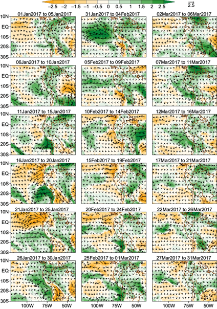
Fig. 8 Five-days anomalies of mixing ratio in 600 hPa (g kg-1, shaded) and anomalies of mixing ratio flux in 600 hPa (vectors).
In upper levels of the troposphere (250 hPa) (Fig. 9) the anomalous configuration of two anticyclonic systems, one north and another south of the equator (better observed between January 31 and February 4) encouraged the positive anomaly of divergence and anomalous easterly winds in the second band of ITCZ near the coastal region and over the north of Peru, similar to Sulca et al. (2017) and the ITCZE configuration and El Niño 1997-1998 pattern found by Takahashi (2004) and in CEN 2017 (Quispe, 2018). In the second half of February a decrease in divergence was observed, related to a decrease of rainfall in the same period; and an increase between March 7-16 associated to a positive anomaly of precipitation was observed (Fig. 5).
5.3. Relationship between precipitation in the Peruvian northwestern region and the formation of the ITCZ second band
Using TRMM monthly precipitation and the Yu and Zhang (2018) methodology (considering Ia < 0.5), we identified eight years with maximum precipitation anomalies to the south of the equator: 1998, 1999, 2000, 2001, 2006, 2009, 2012, and 2017. The majority of these years (80%) coincide with the years found by Yu and Zhang (2018). The differences may be explained by the climatology and the hierarchical clustering used in this research.
With the aim of identifying the daily ITCZ second band formation, we calculated the Ia index considering the areas proposed by Yu and Zhang (2018) (Fig. 10, upper panel) and a new proposed area (Fig. 10, lower panel), and compared them with the daily precipitation gauged in the Bernal coastal station (Fig. 10, middle panel). The first day with an important daily precipitation in Bernal (30 mm) was January 30, and the identification of the ITCZ second band (negative Ia) in new proposed areas was on January 19, 11 days prior to the occurrence of a maximum precipitation. This lag would allow anticipating the occurrence of rain on the coast with more than 10 days of advance; however, this is not possible with the Ia calculated in a total area, which showed a negative value on February 6, one week after the first important daily precipitation in Bernal. This lag may be explained by Sulca et al. (2017), who showed that the integrated moisture transport in periods with positive ITCZE index (ITCZ for the eastern Pacific) is from the west to the east in northwest Peru; as such, the ITCZ second band formation becomes more important in the prediction of rain in that region, especially if it can be identified with days of anticipation.
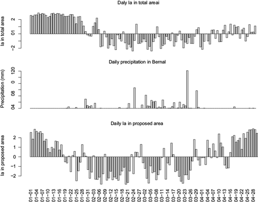
Fig. 10 Upper panel: daily Ia index calculated in total areas (considered in Yu and Zhang, 2018). Middle panel: daily precipitation in the Bernal station (coast of Piura, northwest of Peru). Lower panel: daily Ia index calculated in the new proposed areas.
5.4. Lorenz energy terms
The daily temporal energy analysis (Fig. 11) shows the greatest increase of K E and K Z (K Z is an order of magnitude more than K E , similar to what was found in the ITCZ of the Atlantic by Da Silva and Satyamurti [2013]) in the first half of January, showing an increase of kinetic energy conditions since early January due to the intensification of wind velocity. Other peaks of K E were present in the first half of February and March, but with values close to half of those obtained in January. This decrease in K E can be related to the presence of a CEN event, which was also found by Veiga et al. (2013) and Sátyro and Veiga (2017) in warm ENSO episodes, due to the decrease in the transfer of K E from the environment to the area of the second band, as the warming generated by CEN in the entire eastern Pacific region near Peru did not allow for significant thermal gradients that generate energy transfer. The peaks of K E in the first half of February and March are related to maximums of precipitation in the ITCZ second band (Fig. 5), which can be explained by the increased of convection during this period.
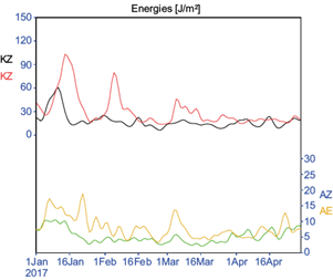
Fig. 11 Time series of volume-integrated Lorenz energy terms (K Z × 104, K E × 103, A Z × 103 and A E × 103) in the SEPn area (values in J m-2).
Values of A Z and A E are smaller than K E and K Z (similar to Da Silva and Satyamurti [2013] for the south Atlantic ITCZ) in the equator regions as the horizontal thermal variations are not significant. The peaks of A E and A Z (the former was greater than the latter) are registered in January and in the first 10 days of March, indicating that, in these days, the thermal gradients in the same latitude were greater than the meridional temperature gradients. Physically, the peaks of A E and A Z on January can be explained by the meridional and zonal thermal gradients in the lower troposphere and sea surface; then, in the first half of March, as it gradually warms up because the CEN occurrence, the convection became important because it generated thermal differences in regions in the same latitude, increasing the values of A E .
Figure 12 shows that among all types of energy conversion, C A (conversion of A Z in A E ) has the smallest order of magnitude, followed by C Z (conversion of K Z in A Z ), which is due to very small horizontal thermal gradients in the ITCZ region. On the other hand, similar to Da Silva and Satyamurti (2013), C E (conversion of A E in K E ) and C K (conversion of K E in K Z ) have the same order of magnitude, as the barotropic instability has a great contribution in equatorial regions.
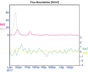
Fig. 12 Time series of volume-integrated energy conversions of the Lorenz energy cycle (C A × 10-2, C Z × 10-1, C K × 100 and C E × 100) in SEPn area (values in W m-2).
The conversion from A E to A Z (negative C A ) in January, in the second half of February and in the second half of March ahead indicates that, due to the northerly motions, the zonal thermal variations slightly increase the thermal gradient between latitudes and generates A Z gain. Contrary, positive C A in the first half of February and March (periods with more convection) indicate transport of warm tropical air to polar latitudes and cold polar air to warm latitudes through meridional motions. This transport could be enhanced by the ascending movements in the convergence zone and subsident movements over southern regions.
The barotropic process (C K ) has high values in January and the first half of February, with positive values indicating conversion from K E to K Z . Considering this process, the increase of K Z observed in the first half of January in Figure 11 is due, mainly, to the energy transferred from the eddies (K E ).
On the other hand, C Z has more variability, mainly in February and March, oscillating between negative and positive values, changing the flux of conversion, manifesting the similar importance of K Z and A Z during the convection of ITCZ second band region. CE has only positive values, with a maximum in the second half of March, indicating that the increase of K E observed in this period in Figure 11 is due to conversion from A E .
At the boundaries, the flux of A Z has the smallest order of magnitude, related to minimum horizontal variations of temperature in the equatorial region (Fig. 13).
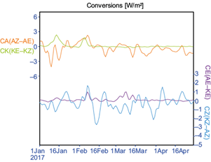
Fig. 13 Time series of volume-integrated boundary energy transports of the Lorenz energy cycle (BA Z × 10-1) in SEPn area (values in W m-2).
The flux of kinetic energy (K Z and K E ) is from the exterior to the area of the ITCZ second band (positive values) in January and the first half of February; as a result, part of maximums of K Z and K E observed in this period were obtained from the environment. During the rest of the period of the study, the transfer of kinetic energy from the boundaries is almost null.
In the case of the flux of A E , almost all values are positive, indicating flux from the exterior to the area of the ITCZ, with a maximum around January 15. While the flux of A Z has values oscillating between positive and negative, indicating, mainly, flux from exterior to the ITCZ second band region in the second half of January, and flux in the opposite direction in the first half of January and early March, possibly due to the greater warming of the ITCZ second band region compared to its surroundings.
6. Summary and conclusions
During the beginning of 2017, the ITCZ second band was present near the coast of northern Peru between the last days of January and the first days of April, with two periods of maximum precipitation during the first half of February and March, which were preceded by positive SST anomalies since January and, mainly, by anomalous north winds and the weakening of the southeast trade winds in a previous period.
A key factor for the development of the second band of the ITCZ is an SST positive anomaly of at least 2 ºC, and at the same time the SST needs to be over 27 ºC, during February and March. However, the determining factor is the behavior of the wind, which must exhibit a constant anomaly from the north (Fig. 4b) and from the west, at least 10 days before the maximum development of precipitation in the second band of the ITCZ.
The behavior of the winds in the ITCZ second band and surroundings were associated with the predominance of an anomalous sea level pressure dipole in the Pacific, with values lower than its normal in the eastern South Pacific (associated with the weakening of the trade winds in the Peruvian coast) and higher than its normal near the equator (from 100 ºW towards the west), generating anomalous west and north winds in the Eastern Pacific near the Peruvian coast.
The mixing ratio in the mid-troposphere had an anomalously positive behavior in the region of the second band of the ITCZ since the last days of January, with a maximum in the first days of February, but with a flow from east to west. However, the change in direction of the flow of the mixing ratio and the positive anomalies over the region (from the Pacific to the continent) occurred only in the first half of March, associated with the development of the maximum convective systems on the northwest coast of Peru. This behavior of flow at medium levels was coupled with the anomalous divergence at high levels, mainly in the region of the ITCZ second band.
The application of the Ia index with daily precipitation and the modified area allows the timely detection of the formation of the ITCZ second band 11 days prior to the occurrence of a maximum precipitation in the Peruvian northwest coast.
According to Lorenz energy terms, the first two peaks of K E (first half of January and second half of February) are related to the boundaries flux from to exterior to the ITCZ second band region. The last peak of K E is related to the conversion from to A E into K E , indicating a change of energy from differential heating in the same latitude to movement, and the values of C K similar to C E show a great contribution of barotropic instability in equatorial regions.

