nueva página del texto (beta)
 Inglés (pdf)
 Artículo en XML
 Referencias del artículo
 Enviar artículo por email
 Citado por SciELO
  Similares en
SciELO
Similares en
SciELO 
 Permalink
Introduction
This paper presents a study of the interaction between operational and credit risk on a small Mexican local credit company using a Fuzzy Gaussian Logistic Credit Score. This research combining a normal logistic regression with a gaussian fuzzy function to analyse the non-standard credit allocation process (due to lack of standards and control in the organization) in a small Mexican credit company. The company’s lack of control and standards gives high autonomy to clerks and managers in different Mexican regions where the leading commercial banks are not giving enough credit.
In the paper, it is calculated the effect of each clerk and branch (operational risk), in terms of basis points, on the interest rate offered by the small credit company, then it estimates the credit Value at Risk for the organization from a fuzzy perspective.
Our paper compares traditional logistic models and the fuzzy version using a ROC curve due to different impacts of the model errors in the firm (a false positive implies a denial of credit; a false positive implies the loss of the borrowed capital and interests). The ROC curve shows that our fuzzy logit model avoids false positives without falling into several false negatives.
There is empirical evidence on the combined negative effect between credit and operational risks Sondakh et. al. (2021), Suryaningsih & Sudirman (2020), Gadzo et. al. (2019), Syafi’i & Rusliati (2016), and Buchory (2015). However, no other papers study the combined effect of operational and credit risks in both the interest rate and the Credit VaR; this allows us to calculate the maximum expected loss in three degrees of uncertainty (Naili & Lahrichi, 2022). This methodology has been called as the Triangular Fuzzy Value at Risk by FG-Logistic Model.
The Fuzzy Gaussian Logistic Credit Score allows calculating the loan’s interest rate by costs, giving a minimum interest rate for each product, and translating into basis points the particularities of each branch or clerk.
In the literature used for this paper, it found several models to forecast the default probability Jacobson & Roszbach (2003) and Pasila et. al. (2017). Furthermore, West (2000) analysed different methods for credit scoring based on the Neural Network Model, concluding that logistic regression is the best model to estimate the credit behaviour. Other similar models are proposed in (Shi et. al., 2022; Liu, 2022; and Li et. al. 2023)
On the other hand, Meghdadi & Akbarzadeh-T (2001) analysed the concept of Probabilistic Fuzzy Logic; this concept is an approach for combining probability theory in fuzzy logic to describe non- deterministic real-world phenomena better.
In general, the methods based on fuzzy theory classify the probability of default as a membership function, allowing to identify degrees of uncertainty that support the non-fuzzy methodology to improve the risk modelling of a credit portfolio (Atalik & Senturk, 2018; Patiño-Pérez et. al. 2015; Pourahmad et. al., 2011b; Sohn et. al. 2016; Hoffmann et. al., 2002; Capotorti, & Barbanera, 2012; Zulkefli et. al. 2019; Liu & Li, 2005; Yu et. al. 2019; Fonseca et. al. 2020; Roy et. al. 2023; Matanda, Eriyoti, & Kwenda, 2022; and Villa-Villa et. al., 2023).
The objective of this research is to model credit risk considering the impact of operational risk, credit product features and customer characteristics, using the proposed fuzzy model. The main hypothesis is that credit risk in a financial institution is a consequence of both the customer and the processes of a financial institution. And as a secondary hypothesis, fuzzy models are claimed to better model the probability of default than traditional econometric methodology.
This research is organized as follows: Section I describes the FG-Logit model for estimating the probability of default, section 2 proposes a Fuzzy Financial Risk Management model. Section 3 presents the analysed credit portfolio forecasts and develops a credit risk assessment. Finally, it discusses conclusions.
Credit scoring and logistic models
Credit score can be defined as a statistical measure of the probability of default of a counterparty. This measure supports decision-making by categorizing creditors through measurable characteristics and matching them with different credit products. Abdou & Pointon (2009) analyses this issue in deep.
By their side, Dinh & Kleimeier (2007) pointed out that the credit score helps minimize credit risk and improves the credit evaluation process, reducing operational risk and the associated expenses. Practitioners heavily use logistic regression because of its adaptability to more comprehensive scoring techniques (Dumitrescu et. al., 2021; Ershadi & Omidzadeh, 2018; Silva et. al., 2018; Sohn et. al., 2016; and Shaw & Ishizaka, 2023).
The Fuzzy Gaussian Logistic Regression Model combines the traditional logistic model with fuzzy theory. It is a fuzzy modification to the traditional logistic model.
Logistic model
The logistic regression model is commonly used to obtain credit scoring parameters. The logistic regression model is a function of conditional probability statementsP(Y = 1|X1, X2, ⋯ Xk) or simply P(X). For more details, see (Kleinbaum & Klein, 2010):
according to (Amemiya, 1985), the maximum likelihood estimator, βi, obtained by maximum likelihood, meets the conditions of consistency and asymptotic normality.
Specifically, the importance of having an efficient model translates into profits for financial institutions. For example, Hai & Ngoc (2020) found that a credit score calculated with the logistic regression model provides up to a 30% increase in profitability.
Fuzzy logistic model
Methods based on fuzzy theory classify the probability of default to identify credit risk according to the customer, loan product, process, and market characteristics. For details, see Ghasemi, et. al. (2023), Atalik & Senturk (2018), Pourahmad et. al. (2011a), Patiño-Pérez et. al. (2015), Pourahmad et. al. (2011b), Sohn et. al. (2016), Hoffmann et. al. (2002), Capotorti, & Barbanera (2012), Zulkefli et. al. (2019), Liu & Li (2005) and Yu et. al. (2019).
In this section, it presents the two methods proposed in our research. The first is the limited dependent variable analysis methodology called Fuzzy Gaussian Logistic Model (FG-Logit); this technique estimates dummy variables as a function of a set of explanatory variables with Gaussian parameters. The second corresponds to calculating various maximum losses by degrees of risk, employing a triangular membership function. This methodology is called as Triangular Fuzzy Value at Risk by FG- Logistic Model.
Fuzzy Gaussian logistic model
This section develops a methodology for analysing limited dependent variables, the “Fuzzy Gaussian Logistic Model” (FG-Logit). The central argument of the model is that the parameters of the traditional Logistic regression follow a Gaussian Membership Function so that it is possible to assign membership values to the coefficients (Figure 1).
Assumption 1. The relationships between P(X) and xi has a membership function
so that
Where xi and P(X) are crisp sets. Then, the FG-Logit model is:
where P(X) is the probability of the event X, xi the independent variables, and μt(βi) represents the fuzzy parameter for each regressor.
Assumption 2. There is a coefficient β∗ inside the membership function μt(βi). Given the min(ε) of the errors estimated by this model. So, P(X) is estimated as a crisp set, if εt has the minimum value provided by (5)
and
where (4) is the membership function of the fuzzy parameter associated with the xi; βi is the average coefficient, estimated through the conventional Logit model by the Maximum Likelihood and δβi is the width of the Gaussian function.
The equation (3) is the Mean Absolute Deviation (MAD), where the dividend is the sum of the mean absolute error, divided by the n events. The errors are measured by (3), the parameter β∗ is estimated by solving the following linear optimization problem:
Subject to
where the width of the curve δβi must be strictly positive, and the parameters βij must be real numbers. Therefore, solving (5), it has that the optimal estimated of FG-Logit is:
Therefore,
Step 1: Define probability of the event as a dependent variable P(X).
Step 2: Establish the independent variables xi.
Step 3: Create the database of dependent and explanatory variables.
Step 4: Estimate the Logistic Model (2).
Step 5: Save Logistic model parameters and use them as the average coefficients βi for the Gaussian membership function.
Step 6: Estimated the FG-Logit.
Minimize (5) from equation (3) and through the membership function (4).
Solve the programming equation (2); where the parameters have a membership function (4) assuming the mean parameter value is the Logit parameter and an arbitrary width of the curve.
Calculate the error (3).
Finally, minimize the errors by modifying the width of the membership function.
Triangular fuzzy credit value at risk by FG-logistic model
According to Guevara & Carrasquilla (2015), the logistic model allows the calculation of the Value at Risk of a credit portfolio. For example, Guerra & Sorini (2020) performed a nonparametric approximation of Value at Risk with fuzzy numbers. In our study, it applies parametric Value at Risk.
where 𝐹 is the confidence level, sigma 𝜎 represents the standard deviation or source of risk, 𝐿𝑃 is the total amount of the loan portfolio, and √𝑡 is the square root of the loan term. It is known as the confidence level, the total amount, and the root of the credit term is costs defined by the financial institution, then:
Assumption 3. The standard deviation σ has a membership function μ(σi), so that is a triangular function μ(σi) ∈ (σLbd , σ, σUbd ).
Assumption 4. Calculate the standard deviations of the loan portfolio σLbd , σ and σUbd using the FG-Logit model. Then the risk sources are:
where,
is the standard deviation of the estimated probability assuming:
Equation (9) shows that βi ∗∗ is equal to the optimal parameter βi ∗ from (8) minus three standard deviations of the membership function (6). The mean value σ is equal to the standard deviation of the probability forecast obtained in (8).
And finally,
is the standard deviation of the estimated probability assuming the modification in the coefficients given in (10):
Equation (9) shows that βi ∗∗∗ is equal to the optimal parameter βi ∗ of (6) plus three standard deviations of the membership function (4).
Therefore, the Triangular Fuzzy Credit Value at Risk for by FG-Logistic Model is:
where (12) indicates the three VaR measures by a triangular membership function.
Fuzzy financial risk management model
This section analyses the credit risk management model proposed in our research. The objective of the Fuzzy Financial Risk Management Model is to minimize credit risk by defining the risk rate that financial institutions face because of their business process.
This method uses the FG-Logit model to obtain the parameters that recognize the effect of the regressors and assess the probability of default. The proposed risk management model consists of three fundamental phases:
Construct a credit score and parametrize the independent variables.
Obtain the risk rate per variable and calculate the Credit Value at Risk.
Calculate the interest rate by expenses, assuming the dividends.
The first phase allows financial institutions to define credit risk and establish a credit score that predicts a customer’s default probability based on the customer’s characteristics, origination branch, and market environment.
The second phase provides specific information on branches, credit operators, credit purposes, and other variables related to the credit product that change default probability. Finally, it calculates the minimum interest rate applied by the financial institution to its loan product. This phase allows the institution to reduce the loan product rate originated by credit origination issues.
Defining the interest rate of a credit product through expenses
It should point out that the FG-Logit technique and the Fuzzy VaR are taken up again as a fundamental part to elaborate this credit risk management methodology. Next, it describes the steps to get the Fuzzy Financial Risk Management Model (figure 2).
Step 1. Define the event of default: The institution must consider its internal policies, financial market regulations, type of loan product, delinquency, or other appropriate sources of risk.
Step 2. Establish the values of the independent variables and create the database of dependent and explanatory variables.
Use binary values to establish independent variables for branches and credit executives. Steps 3 and 4 correspond to the estimation of the FG-Logit model presented in section 1.2.
Step 3. Estimate a logistic model and save its parameters.
Step 4. Estimate the Fuzzy Gaussian Logistic model.
Step 5. Select a decision threshold (DT); it used the probability of default (PD) between 60% and 80%. C
If the estimated probability exceeds the threshold, it will label the loan as delinquent.
Once it selects the model, it rejects any probability outside these thresholds.
where rCR is the credit risk rate of the total loan portfolio, PD̂i is the estimated probability of default on loan i, LAi is the loan amount of credit i, and LA represents the institution’s total loan portfolio. The estimated risk rate is the risk cost of its customers and counterparties associated with each regressor.
Step 7. Determine the increase in the risk rate caused by each executive or branch.
Step 8. Create a new estimate of the probability of default; it assumes that the information of one credit executive is equal to zero and reapply the step 4 to determine the new probability of default for every executive.
To make other estimates of the probability of default, it assumes that the information of one branch is equal to zero and reapply the step 5 to determine the new probability of default of each branch analysed.
then
To make other estimates of the probability of default, it assumes that the information of one branch is equal to zero and reapply the step 5 to determine the new probability of default of each branch analysed.
then
and
where r′CR is the risk rate generated by each loan officer, so the methodology allows us to identify the specific risk rate. On the other hand, r′′CR indicates the risk rate per branch, so two scenarios can be generated. The first corresponds to an increase in credit risk, so the institution must monitor the causes of this increase and make decisions to improve the process, diagnosis, and minimization of losses.
where: Administrative expense (rae), Credit Risk (rcr), Dividends (rd), 10% in our paper, and Funding expense (rfe).
Data description
The database uses the commercial credits originated by a Mexican small credit organization (SOFIPO) between December 2015 - June 2018 in eight branches and considering twelve credit executives.
The organization provided the data under a Non-Disclosure Agreement, so it cannot provide further information about the loans or their originator.
The original database contained 138 variables, but the final model uses only 33 (see table 1).
Table 1 Numerical description of the independent variables
| Variable | Type | Maximum | Minimum |
|---|---|---|---|
| Food Industry | Binary | 1 | 0 |
| Credit Executive 03 | Binary | 1 | 0 |
| Credit Executive 04 | Binary | 1 | 0 |
| Credit Executive 06 | Binary | 1 | 0 |
| Credit Executive 09 | Binary | 1 | 0 |
| Credit Executive 11 | Binary | 1 | 0 |
| Credit Executive 12 | Binary | 1 | 0 |
| Loan Amount¹ | Continuous | 1000 | 4 |
| Cattle breeding | Binary | 1 | 0 |
| Credit Product 01 | Binary | 1 | 0 |
| Age² | Continuous | 83 | 20 |
| Retail Business | Binary | 1 | 0 |
| Purpose credit 02 | Binary | 1 | 0 |
| Purpose credit 03 | Binary | 1 | 0 |
| Purpose credit 04 | Binary | 1 | 0 |
| Brick factory | Binary | 1 | 0 |
| Stockyard maintenance | Binary | 1 | 0 |
| Manner of payment | Binary | 1 | 0 |
| Instalment Payments³ | Continuous | 60 | 6 |
| Ornament Production | Binary | 1 | 0 |
| Payment amount⁴ | Continuous | 270 | 30 |
| Pig farming | Binary | 1 | 0 |
| fixed asset loans | Binary | 1 | 0 |
| Business services | Binary | 1 | 0 |
| Individual Services | Binary | 1 | 0 |
| Gender⁵ | Binary | 2 | 1 |
| Branch 01 | Binary | 1 | 0 |
| Branch 03 | Binary | 1 | 0 |
| Branch 05 | Binary | 1 | 0 |
| Branch 06 | Binary | 1 | 0 |
| Branch 08 | Binary | 1 | 0 |
| Credit duration in years | Continuous | 5 | 1 |
Source: Own elaboration with information from an anonymous financial institution.
On the other hand, it defined the probability of default as a binary variable. The values assigned to each of the loans analysed are as follows:
Number one is assigned when the loan default (more than 180 days past due).
It places zero for recovered loans.
Once the probability of default was classified, it found that of the 3,383 loans granted, 363 defaulted.
Fuzzy credit score: The application model
This section develops a comparative analysis of different probabilistic models. Based on the variables described above, the probability of loan default is estimated using Logit, Probit, Extreme Values, Pattern Recognition Neural Network, and FG-Logit models.
The analysis of the explanatory variables involved the omitted and redundant variables test; this resulted in the best model for estimating the probability of default.
The coefficients of the four parametric models analysed (Table A1) show that the influence of the explanatory variables on the probability of default is statistically significant for the 38 attributes used. However, it must point out that the FG-LOGIT model increases the magnitude of the impact of each variable in different directions on the line of real numbers.
First, we obtained increases in the magnitude of the coefficient but maintained the same sign. In other words, the explanatory variables estimate a more significant impact on the probability of default compared to traditional models. Such is the case for the credit purposes of the brick factory, stockyard maintenance, ornament production, and pig farming.
Second, the proposed methodology preserves the estimated parameter value at the same level. Therefore, it assumes that the membership function of the fuzzy coefficients is within the confidence interval of the non-fuzzy parameters, for example, in the specific case of the attributes of the cattle breeding, purpose credit 02, credit executive 12, and branch 08.
Finally, it found the change in the sign of the fuzzy coefficient compared to that estimated by traditional models; this shows that the risk measurement derived from the membership function allows capturing information unobserved by non-fuzzy methodologies. In other words, the proposed model identifies contrary scenarios than those indicated by other methodologies, allowing to define the risk of the variables in a more accurate way; it can observe this in the coefficients of the food industry, business services, credit duration in years, and gender.
The marginal effects analysis shows the impact of the variables on the probability of default of the loan product examined. Table 2 compares the slopes of the parameters associated with the models applied in our study.
Table 2 Comparison of the marginal effects for the credit purpose variables
| The slope of Model Parameters | ||||
|---|---|---|---|---|
| Variable/Model | Probit | Logit | Extreme Values | FG-Logit |
| Food Industry | 0.20 | 0.35 | 0.20 | -2.09 |
| Cattle breeding | 0.06 | 0.13 | 0.06 | 0.05 |
| Credit Product 01 | -0.34 | -0.67 | -0.25 | -5.01 |
| Retail Business | 0.17 | 0.31 | 0.16 | 1.18 |
| Purpose credit 02 | 0.07 | 0.12 | 0.07 | 0.04 |
| Purpose credit 03 | 0.37 | 0.69 | 0.32 | 9.55 |
| Purpose credit 04 | 0.13 | 0.19 | 0.14 | 4.63 |
| Brick factory | 0.35 | 0.61 | 0.33 | 0.55 |
| Stockyard maintenance | 0.09 | 0.15 | 0.11 | 7.41 |
| Ornament Production | 0.16 | 0.30 | 0.14 | 1.08 |
| Pig farming | 0.52 | 1.07 | 0.41 | 0.90 |
| Fixed asset loans | 0.24 | 0.44 | 0.23 | 8.78 |
| Business services | 0.05 | 0.06 | 0.09 | -1.96 |
| Individual Services | 0.35 | 0.69 | 0.31 | 6.93 |
| Credit Executive 03 | -0.08 | -0.16 | -0.06 | -2.46 |
| Credit Executive 04 | -0.22 | -0.42 | -0.20 | -4.24 |
| Credit Executive 06 | -0.18 | -0.31 | -0.17 | -0.25 |
| Credit Executive 09 | 0.13 | 0.22 | 0.14 | 3.70 |
| Credit Executive 11 | 0.16 | 0.28 | 0.18 | 12.74 |
| Credit Executive 12 | -0.17 | -0.32 | -0.15 | -0.26 |
| Branch 01 | 0.10 | 0.20 | 0.09 | 10.14 |
| Branch 03 | 0.18 | 0.37 | 0.15 | 2.37 |
| Branch 05 | 0.11 | 0.22 | 0.10 | 9.04 |
| Branch 06 | 0.44 | 0.85 | 0.41 | 20.96 |
| Branch 08 | 0.15 | 0.30 | 0.11 | 0.26 |
| Loan Amount | 0.00 | 0.00 | 0.01 | 0.03 |
| Instalment Payments | -0.00 | -0.01 | -0.01 | -0.18 |
| Credit duration in years | 0.04 | 0.09 | 0.03 | -2.14 |
| Age | -0.00 | -0.01 | -0.01 | -0.21 |
| Gender | -0.03 | -0.03 | -0.03 | 0.89 |
| Manner of payment | 0.05 | 0.10 | 0.03 | 2.62 |
Source: Own elaboration.
The table above shows the effect of each OCF the variables analysed on the probability of default. For example, if the purpose of a loan is the food industry, according to the Probit, Logit, and Extreme Value models, the probability of default increases by 0.20, 0.35, and 0.20, respectively. On the other hand, the FG-Logit shows an opposite result because it indicates a default probability decreases by 2.09 for these loans, as seen in the sign.
In general, it can observe that the marginal effect provided by the FG-Logit model (in absolute value) is significantly higher than those of the traditional models. This result is a consequence of the fact that traditional models (Probit, Logit, and Extreme Values) estimate the average effect of each variable on the probability of default. On the other hand, the fuzzy methodology examines different scenarios in the membership function of the parameters of each variable, which results in a better approximation of the loans that defaulted.
Therefore, the FG-Logit methodology presents more significant marginal effects because it captures both the average impact and the events at the extremes of the credit probability of default distribution function.
Efficiency analysis of limited dependent variable models
The previous section examined the proposed credit scoring models’ estimation results, which raises the following questions: Which of the models generates the best estimation results? Moreover, what is the best methodology for designing a credit score?
The answers to these questions are presented in this section through several tests to measure and compare the efficiency of the models with limited dependent variables by graphical tests (figures B1, B2, B3, B4, and B5). The methodologies used are the mean absolute error, the confusion matrices (tables C1, C2, C3, C4, C5, D1, D2, D3, D4, and D5), and the ROC curve.
Table 3 illustrates the mean absolute error of the five models implemented. it shows three columns of results for each model, which refer to the evaluation of the forecasts on the total portfolio (PD), when the loan defaulted (PD=1), and the recovered loans (PD=0). This test indicates that the best model is the one that provides the lowest forecast error.
Table 3 Mean absolute deviation comparison
| Model | PD | PD=1 | PD=0 |
|---|---|---|---|
| n=3383 | n=363 | n=3020 | |
| Probit Model | 6.72% | 30.04% | 3.92% |
| Logistic Model | 6.35% | 29.20% | 3.60% |
| Extreme Values Model | 7.49% | 34.11% | 4.28% |
| Pattern Recognition Neural Network Model | 5.63% | 25.41% | 3.26% |
| Fuzzy Gaussian Logistic Model | 3.25% | 23.95% | 0.76% |
Source: Own elaboration
The model with the lowest mean absolute error is the FG-Logit model, followed by the neural network; this indicates that the model proposed in this research is the most suitable for forecasting the probability of default of the loan portfolio. Therefore, the fuzzy methodology is the one that best recognizes the loans with the highest probability of recovery and default.
It should be note that the methods for measuring estimation efficiency have specific characteristics. For example, the confusion matrix and ROC curve must accurately classify which forecast meets the classification criteria, so two selection thresholds are proposed (figure 3).
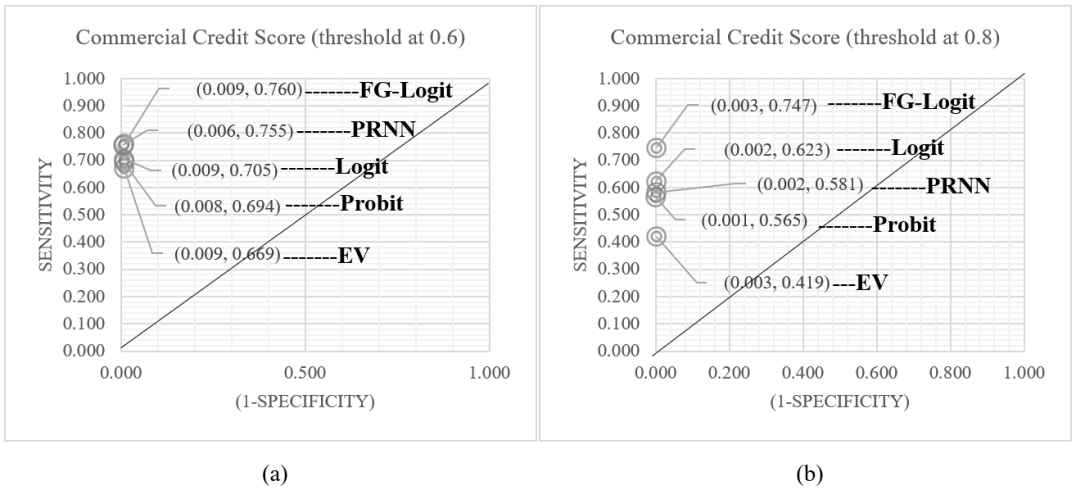
Source: Own elaboration.
Figure 3 Comparison of ROC Curve. (a) depicts the models’ rank in the space of the ROC curve at a threshold of 60% probability of default.; (b) describes the models’ rank in the space of the ROC curve at a threshold of 80% probability of default.
According to the results, the fuzzy model is the one that best recognizes the characteristics of defaulted and recovered loans, and this was true at both thresholds implemented. In addition, the FG-Logit methodology had no significant impacts in the face of threshold shifts.
Credit risk rate
The previous sections have shown that the most appropriate model for measuring credit risk is the FG- Logit, so it calculates the risk rate faced by the financial institution for this credit product. Within the risk management model, the calculation of the credit risk rate corresponds to step 6. Therefore, it uses (14) to determine the results of this section.
Table 4 shows the comparison between the financial institution’s risk rate against the FG-Logit estimate. It can observe a difference of 1.56%; in this aspect, the proposed model underestimates the credit risk but with a relatively low error. Therefore, continuing with the next steps of the credit risk management model with an estimate of 16.4%.
Impact of operational risk on the credit risk rate caused by credit executives and branches
Our research analyses the impact of credit operations on credit risk behaviour. Therefore, the proposed risk management tool incorporates step 9 (estimation of the credit agent and branch risk rate).
Therefore, it develops an analysis of the risk rate of each of the variables associated with operational risk. It assesses each executive and branch’s impact on the general process. It performs the calculations of the estimated interest rate impact for the credit product using this methodology.
Table 5 indicates that the credit evaluation process performed by these officers presents some external or internal variable that motivates an increase in credit risk. However, the information provided by our model does not allow us to know why this increase occurs, but it provides the necessary guidance for a more in-depth evaluation in terms of credit process, market, or other variables related to the evaluation of the credit product.
Table 5 The estimated increase in the interest rate per credit executive by the FG-Logit model
| Credit executive | Estimated risk rate |
|---|---|
| Credit Executive 03 | -0.06% |
| Credit Executive 04 | -0.03% |
| Credit Executive 06 | 0.00% |
| Credit Executive 09 | 0.81% |
| Credit Executive 11 | 1.39% |
| Credit Executive 12 | 0.00% |
Source: Own elaboration.
The operations of the branches at the financial institution are fundamental to the proper execution, evaluation, and recovery of a loan product. Table 6 shows that the general processes carried out in branches must also be standardized. Therefore, staff must have minimum criteria to carry out their activities to ensure the best results.
Triangular fuzzy value at risk
The definition of maximum loss is one of the main concepts measured in risk management theory. It identifies the maximum amount that a financial institution can lose from its lending activities.
The Fuzzy Triangular Value at Risk (table 7) method provides the expected loss for three degrees of uncertainty. In other words, VaR recognizes the market volatility and uncertainty; this gives a range to define the best VaR measure to establish risk provisions.
Determination of the interest rate of a credit product through expenses
The last section of our research corresponds to the definition of the minimum interest rate to apply to the expense loan product. This calculation is the step of the fuzzy risk management model presented in the previous sessions. The risk identification and overhead costs are the methodology’s base.
Table 8 shows the term structure of the interest rate proposed by our methodology, whose components correspond to the expenses incurred by the institution and which it is obliged to recover through the interest rate of the loan product. The terms correspond from one day to 5 years, considering the essential characteristics of the interest rate. In other words, the starting point for determining the interest rate of the loan product is the annualized rate of expenses.
Table 8 Components of the term structure of interest rates per expense for the credit product
| Expense item\ term | 1 day | 30 days | 90 days | 180 days | 1 year | 2 years | 3 years | 4 years | 5 years |
|---|---|---|---|---|---|---|---|---|---|
| Administrative expense | 0.02% | 0.74% | 2.21% | 4.42% | 8.83% | 8.83% | 8.83% | 8.83% | 8.83% |
| Credit risk | 0.05% | 1.37% | 4.10% | 8.20% | 16.40%6 | 22.76% | 29.11% | 35.46% | 41.82% |
| Dividends | 0.03% | 0.83% | 2.50% | 5.00% | 10.00% | 20.00% | 30.00% | 40.00% | 50.00% |
| Funding expense | 0.00% | 0.10% | 0.30% | 0.60% | 1.21% | 2.42% | 3.63% | 4.84% | 6.05% |
| Interest Rate | 0.10% | 3.04% | 9.11% | 18.22% | 36.45% | 54.01% | 71.57% | 89.14% | 106.70% |
Source: Own elaboration with data from (2015-2018) the National Banking and Securities Commission (Spanish acronym, CNBV).
Administrative expenses are the first element to be incorporated into the interest rate. For calculating these expenses, the entity’s financial statements are used, from which the information relating to the loan product is extracted and calculated by dividing the administrative expenses by the total value of the assets under management.
Discussion
Risk management in financial institutions became important given the financial market volatility, the unavailability of good risk measurement, and the inherent uncertainty of the financial sector; consequently, it needs to develop more efficient and accurate tools to comprehend the financial risks.
For this reason, our research presents a new technique for Credit Risk management called Fuzzy Gaussian Logistic Credit Score. In addition, derived from the proposed methodology, it develops two methodologies for risk management and interest rate definition.
The first one corresponds to the Value at Risk measurement by possibility intervals. In other words, it is possible to calculate the maximum expected loss in three degrees of uncertainty through a triangular membership function. It called this approach as Triangular Fuzzy Value at Risk by FG-Logistic Model.
Furthermore, the second corresponds to calculating the interest rate of a credit product by expenses. In other words, it estimates the interest rate using the administrative expense, risks, dividends, and funding expenses. This process makes it possible to define a minimum rate for a lending institution for a credit product.
It compares Probit, Logit, Extreme Values, and Pattern Recognition Neural Network against the modified fuzzy logic technique, which generated the following results: First, the proposed model provides a new assignment of the degree of influence of the explanatory variables on the probability of default of a loan, measured through the coefficients. Thus, it shows that the level of risk of the variables increased, decreased, or remained close to the Logit coefficients.
Conclusions
In conclusion, the benefits provided by our methodologies in the first instance are for the continuous improvement of risk management, promoting a better reading of uncertainty. Also, the results of the fuzzy techniques of this study provide better information for financial decision-making, which provides new instruments in the field of credit risk study. Moreover, with this, the improvement of the credit activity of our economy, in other words, the most significant benefits are obtained by the credit seekers because a better administration translates into lower costs and greater possibilities of acquiring a loan.
This research found that the FG-Logit model can modify the sign of the variable, showing that in the minimum forecast error, there is the possibility that the risk of a variable is opposite to that provided by traditional methodologies.
Consequently, the FG-Logit model provides a more specific scenario for each source of risk, caused by a better estimation of the behaviour of the variables related to the credit process. The first relevant conclusion is that the parameter associated with each independent variable can generate three scenarios:
First, it found that the coefficient stabilizes at similar levels or is modified in a minimal proportion, indicating that the fuzzy logic-based model identifies that the Logit efficiently captures the risk of the variable.
Second, the value of the coefficient varies significantly, increasing or decreasing the impact; this means that the FG-Logit model indicates that the traditional Logit model does not correctly estimate the information of the variable. Therefore, the magnitude of the variable’s influence on the probability of default changes significantly.
Finally, the parameter changes sign, indicating that the fuzzy model identifies that the risk of the variable is inverse to that estimated by the Logit model; that is, the least error criterion provides information that the logistic regression analysis does not recognize.
Additionally, it recognizes that several variables and indicators influence credit risk. One of them is the financial institution’s operation, which significantly influences the default probability. On the other hand, the purpose of the loan is of utmost importance to determine cash flows and the borrower’s payment capacity, to which our methodology recognizes there is a variety of defects, and depending on the economic activity, the risk can be high or low.
In addition, it identified that the structure of the loan product also influences the probability of default, although to a lesser extent than the previous indicators. Finally, client characteristics also influence loan default, especially credit history.
The results of our study provide three new methodologies which stand out for their higher efficiency compared to other models. The FG-Logit model presented higher efficiency than traditional models and provided new information to the analysis and management of the loan portfolio.
The Fuzzy Financial Risk Management model is an integrative methodology that recognizes all the risks faced by a financial institution and measures them in such a way as to provide a value for the risk rate for each of the variables associated with the credit process. The result is the interest rate per expense.
The Triangular Fuzzy Value at Risk method provides the expected loss for three degrees of uncertainty. In other words, it recognizes the VaR with low volatility in the market, average risk, and high levels of uncertainty; this provides a range to define the best VaR measure for establishing risk provisions.
In recent months, financial market uncertainty has increased to unprecedented levels. Therefore, it is essential to have better methodologies to guide us in making decisions to minimize the risk exposure of financial assets.
Therefore, the fuzzy theory risk management methods proposed in this study support improving the design of policies, measures, and strategies to manage credit risk; this not only helps to improve the financial performance of the financial institution but also to lower the cost of debt so that customers can borrow at a rate that tends to be lower and lower.