


 nueva página del texto (beta)
 Inglés (pdf)
 Artículo en XML
 Referencias del artículo
 Enviar artículo por email
 Citado por SciELO
  Similares en
SciELO
Similares en
SciELO 
 Permalink
Introduction
Harry Markowitz developed the theory of mean-variance portfolio optimization (Markowitz, 1952). Theory widely accepted in the literature (Nobel Prize 1990). Markowitz (1959) defines semi-variance to measure only negative deviations as an alternative measure of portfolio risk.
Regardless of market conditions and under the arbitrage-free condition, Jin et al. (2006) showed that efficient single-period semi-variance strategies are superior to mean-variance strategies. Because the variance penalizes deviations above/below the mean equally. There can be three ways to obtain the semi-variance (1) deviation below an expected or average value, (2) deviation below zero and (3) deviation below a target. This paper empirically studies (3), where the target is the annual return of the DJIA.
A study similar to the one presented in this paper is Ortiz-Ramirez et al. (2019). They analyze 100 portfolios with different configurations using 12 assets from the Mexican Stock Exchange, between 2015 to 2017. They found that semi-variance and mean absolute deviation present higher returns compared to mean-variance or maximum Sharpe portfolios. In this paper, the 30 assets that component the DJIA index are used and held over a one-year period. The same is done every day from 2000 to 2020. 5 134 observations of annual yields are used. These results are discussed in the following sections.
The use of semi-variance has been shown to have important predictive qualities for future market volatility (Barndorff-Nielsen, 2008). Estrada (2003) mentions that the mean semi-variance is correlated with the expected utility and the utility of the average compound return. Grootveld & Hallerbach (1999) empirically tested different portfolios (US asset allocation) with various risk measures that consider the downward deviation or semi-variance. The return differential with portfolios using mean-variance was slightly higher than bond returns. Several authors (Lari-Lavassani & Li, 2003; Pla-Santamaria & Bravo, 2013; Grootveld & Hallerbach, 1999; Barndorff-Nielsen, 2008; Ortiz-Ramirez et al., 2019; Rutkowska-Ziarko & Garsztka, 2014) conclude that portfolio optimization using semi-variance is more appropriate than mean-variance. Since minimizing only downside risk or portfolio loss can be achieved by semi-variance optimization, but not by mean-variance.
There are authors who not only use semi-variance to optimize portfolios, but also to select assets or as part of the variables to be considered for portfolio allocation. Garkaz (2011) use a genetic algorithm with different frequencies of observations for the purpose of selecting and optimizing portfolios. Rutkowska-Ziarko (2013) uses a synthetic indicator for each company, describing its economic and financial situation that allows finding a fundamental portfolio with the minimum semi-variance. Barati et al. (2016) use multi-period models of portfolio selection based on the average semi-variance. Chang et al. (2009) uses a genetic algorithm with different risk measures: variance-mean, semi-variance, mean absolute deviation and variance with skewness. Dzuche et al. (2020) use a trapezoidal and triangular fuzzy variable based on expected value, variance, semi-variance, skewness, kurtosis and semi-curtosis to optimize portfolios. Huang (2008) proposes two fuzzy models that use semi-variance as an alternative for portfolio construction, without making comparisons with other models in the literature. In this paper, we will not use fuzzy numbers.
This study is similar to Pla-Santamaria & Bravo (2013) who seek to design portfolios for banking clients with the objective of minimizing the deviation below the average (mean semi-variance). Companies categorized as "Blue Chips" are used. Companies that in times of financial crisis would be expected to be more stable than the rest of the stocks in the market. The shares of the Dow Jones Industrial Average components are taken with daily frequency in the period 2005-2009, weekly returns and diversification restrictions so that each weight (in each asset) is less than 5%. In our study the period is between 2000-2020 with annual returns, different investment restrictions are studied for each asset and the semi-variance is with respect to the performance of the DJIA. The results of Pla-Santamaria & Bravo (2013) favor portfolio allocation using mean semi-variance since it reflects downside risk. Similarly, Estrada (2007) mentions that semi-variance is a better measure of variance compared to modern portfolio theory.
In more recent studies. Kumar et al. (2022) compare minimum-variance, semi-variance, equal-weight and maximum-return portfolios. The first two portfolios outperform the rest in terms of expected returns and lower risks, with the semi-variance being the portfolio with the lowest expected risk and the highest Sharpe ratio. Ravinesh et al. (2022) by comparing equally weighted portfolios, mean-variance, and semi-variance. The semi-variance excels in terms of profitability and a better Sharpe ratio. Cheng et al. (2022) obtain a better asset allocation by minimizing the semi-variance, by the inverse distribution of uncertainty. This paper the optimization of the semi-variance is performed as the original authors. Also, in the literature we can find the use of artificial intelligence to improve portfolio optimization. Manzoor & Nosheen (2022) using Artificial Neural Networks and return forecasting seek to optimize portfolios of assets from the benchmark index with lower semi-variance. Whose results were better than equally weighted portfolios. Ma et al. (2022) optimize semi-variance portfolios using reinforcement learning and semi-variance. In the previous studies, it is unclear whether the use of optimization methods or artificial intelligence was better than investments in assets that replicate the benchmark index. The following sections attempt to answer this question.
The predictive power of semi-variance has also been studied. Ismail et al. (2022) seek to predict the occurrence of financial distress by predicting downside risk or semi-variance. Evaluating financial distress as negative equity and/or equity less than 25% of issued and paid-up capital. They concluded that semi-variance is positively significant in explaining financial distress for both cases. This paper does not attempt to predict the semi-variance, but to find the best combination of assets that decrease the semi-variance in the portfolio. The evaluation is done with the appraisal, where the DJIA is the portfolio to beat. The appraisal helps us to adjust the risk of the portfolios to compare them with each other.
Although the literature shows the consideration of semi-variance over variance because semi-variance only considers movements below a target, while variance considers risk both positive and negative returns, without considering a target. Some questions remain unanswered, or the answer is not clear. Using the semi-variance to weigh the components of an index, would we have as a result a better risk-return relationship? The literature compares mean-variance vs. semi-variance, but never compares against index investing, how likely am I to outperform the index? What would be the average return differential? What investment constraints are best to optimize portfolios (asset allocation)?
These questions are answered in the following three sections: methodology, results, and conclusions.
Methodology
The following passive strategies are tested empirically: (1) maintaining the investment in the DJIA for one year (252 trading days), (2) building an investment portfolio with the components of the DJIA for one year, optimizing the portfolio with the minimum mean-variance, (3) building an investment portfolio with the components of the DJIA for one year, with the same weighting in each asset, (4) building an investment portfolio with the components of the DJIA for one year, optimizing the portfolio with the minimum semi-variance. Where the semi-variance is the lower of zero or the one-year asset return spread minus the one-year DJIA return. During each consecutive day (5 134 observations) for each type of passive strategy. The portfolios were simulated with the following optimization algorithm.
Subject to
For the mean-variance asset allocation
For the equal weighted asset allocation
For the semi-variance asset allocation
r = annual return
252 observations of previous annual returns of each component of the DJIA were taken to perform the optimization, where the percentages to be invested in each asset were obtained. The result of the optimization was maintained up to 252 trading days, regardless of whether the DJIA changed or not. A total of 5 134 optimizations were performed for each strategy (mean-variance and semi-variance). Ibrahim & Eldomiaty (2007) calculate the semi-variance using the mean of the returns instead of a benchmark, since it produces normal distributions in the returns and thus meets the assumptions of normality in the optimization models. In this paper, the model is tested with out-of-sample data to validate the model, without seeking to meet normality in the results. Held et al. (2020) study the variance risk premium, using semi-variance, we find that the variance premium is driven almost exclusively by downward movements. In this paper, we will use the premiums only for the appraisal calculation.
To verify that each day the components of the DJIA are taken into account to assemble the portfolios. The above algorithm verifies the dates shown in Table 1 where there is a change in the DJIA components, and thus updates the 30 components at each moment. Table 6 shows the components that the DJIA had between 2000-2020. Asset prices between January 13, 1998, and May 28, 2021, were used (source FactSet).
Table 1 Changes in the components of the Dow Jones Industrial Average: 2000-2020.
| 1 | 01/11/1999 | 6 | 08/06/2009 | 11 | 01/02/2018 |
| 2 | 08/04/2004 | 7 | 24/09/2012 | 12 | 26/06/2018 |
| 3 | 21/11/2005 | 8 | 23/09/2013 | 13 | 02/04/2019 |
| 4 | 19/02/2008 | 9 | 19/03/2015 | 14 | 06/04/2020 |
| 5 | 22/09/2008 | 10 | 01/09/2017 | 15 | 31/08/2020 |
Source: FactSet. For more details, see the appendix.
Table 2 Mean-variance Portfolio vs. DJIA (2000-2020)
| Maximum
percentage to be invested in each asset |
Probability
of annual return > DJIA |
Average
annual return DJIA |
Average
annual return Mean-variance |
Standard
deviation DJIA |
Standard
deviation Mean-variance |
Mean-variance
(Return / volatility) |
DJIA
(Return / volatility) |
| 5.0% | 44.9% | 6.3% | 5.5% | 14.9% | 14.6% | 0.38 | 0.42 |
| 10.0% | 41.0% | 6.3% | 4.9% | 14.9% | 13.3% | 0.37 | 0.42 |
| 15.0% | 41.4% | 6.3% | 4.7% | 14.9% | 12.9% | 0.36 | 0.42 |
| 20.0% | 41.8% | 6.3% | 4.7% | 14.9% | 12.9% | 0.36 | 0.42 |
| 25.0% | 42.2% | 6.3% | 4.8% | 14.9% | 13.0% | 0.37 | 0.42 |
| 30.0% | 42.7% | 6.3% | 4.8% | 14.9% | 13.2% | 0.37 | 0.42 |
| 35.0% | 42.5% | 6.3% | 5.0% | 14.9% | 13.4% | 0.37 | 0.42 |
| 40.0% | 42.4% | 6.3% | 5.0% | 14.9% | 13.5% | 0.37 | 0.42 |
| 45.0% | 42.1% | 6.3% | 5.1% | 14.9% | 13.7% | 0.37 | 0.42 |
| 50.0% | 42.0% | 6.3% | 5.1% | 14.9% | 13.7% | 0.37 | 0.42 |
| 55.0% | 42.0% | 6.3% | 5.1% | 14.9% | 13.8% | 0.37 | 0.42 |
| 60.0% | 42.1% | 6.3% | 5.1% | 14.9% | 13.9% | 0.37 | 0.42 |
| 65.0% | 42.2% | 6.3% | 5.1% | 14.9% | 14.1% | 0.36 | 0.42 |
| 70.0% | 42.3% | 6.3% | 5.1% | 14.9% | 14.2% | 0.36 | 0.42 |
| 75.0% | 42.4% | 6.3% | 5.1% | 14.9% | 14.3% | 0.36 | 0.42 |
| 80.0% | 42.6% | 6.3% | 5.1% | 14.9% | 14.4% | 0.36 | 0.42 |
| 85.0% | 42.7% | 6.3% | 5.1% | 14.9% | 14.6% | 0.35 | 0.42 |
| 90.0% | 42.8% | 6.3% | 5.2% | 14.9% | 14.7% | 0.35 | 0.42 |
| 95.0% | 42.8% | 6.3% | 5.2% | 14.9% | 14.9% | 0.35 | 0.42 |
| 100.0% | 42.8% | 6.3% | 5.2% | 14.9% | 14.9% | 0.35 | 0.42 |
Source: own elaboration and data from FactSet.
Table 3 Equal-weighted Portfolio vs. DJIA (2000-2020)
| Percentage
to be invested in each asset |
Probability
of annual return > DJIA |
Average
annual return DJIA |
Average
annual return Equal-weighted |
Standard
deviation DJIA |
Standard
deviation Equal-weighted |
Equal-weighted
(Return / volatility) |
DJIA
(Return / volatility) |
| 3.3% | 51.1% | 6.3% | 6.4% | 14.9% | 16.2% | 0.39 | 0.42 |
Source: own elaboration and data from FactSet.
Table 4 Semi-variance Portfolio vs. DJIA (2000-2020)
| Maximum
percentage to be invested in each asset |
Probability
of annual return > DJIA |
Average
annual return DJIA |
Average
annual return Semi-variance |
Standard
deviation DJIA |
Standard
deviation Semi-variance |
Semi-variance
(Return / volatility) |
DJIA
(Return / volatility) |
| 5.0% | 60.6% | 6.3% | 6.6% | 14.9% | 15.2% | 0.438 | 0.42 |
| 10.0% | 63.2% | 6.3% | 6.6% | 14.9% | 15.1% | 0.440 | 0.42 |
| 15.0% | 65.2% | 6.3% | 6.5% | 14.9% | 15.1% | 0.429 | 0.42 |
| 20.0% | 62.2% | 6.3% | 6.5% | 14.9% | 15.0% | 0.435 | 0.42 |
| 25.0% | 61.5% | 6.3% | 6.6% | 14.9% | 15.0% | 0.438 | 0.42 |
| 30.0% | 61.7% | 6.3% | 6.7% | 14.9% | 15.1% | 0.442 | 0.42 |
| 35.0% | 61.7% | 6.3% | 6.6% | 14.9% | 15.0% | 0.443 | 0.42 |
| 40.0% | 61.3% | 6.3% | 6.7% | 14.9% | 15.0% | 0.444 | 0.42 |
| 45.0% | 60.8% | 6.3% | 6.7% | 14.9% | 15.0% | 0.445 | 0.42 |
| 50.0% | 60.6% | 6.3% | 6.7% | 14.9% | 15.0% | 0.447 | 0.42 |
| 55.0% | 60.3% | 6.3% | 6.7% | 14.9% | 15.0% | 0.449 | 0.42 |
| 60.0% | 60.1% | 6.3% | 6.8% | 14.9% | 15.0% | 0.450 | 0.42 |
| 65.0% | 60.4% | 6.3% | 6.8% | 14.9% | 15.2% | 0.451 | 0.42 |
| 70.0% | 60.9% | 6.3% | 6.9% | 14.9% | 15.2% | 0.452 | 0.42 |
| 75.0% | 61.6% | 6.3% | 6.9% | 14.9% | 15.3% | 0.454 | 0.42 |
| 80.0% | 61.7% | 6.3% | 6.9% | 14.9% | 15.3% | 0.453 | 0.42 |
| 85.0% | 61.0% | 6.3% | 6.9% | 14.9% | 15.5% | 0.446 | 0.42 |
| 90.0% | 60.2% | 6.3% | 6.8% | 14.9% | 15.5% | 0.442 | 0.42 |
| 95.0% | 59.5% | 6.3% | 6.8% | 14.9% | 15.5% | 0.440 | 0.42 |
| 100.0% | 58.6% | 6.3% | 6.7% | 14.9% | 15.5% | 0.433 | 0.42 |
Source: own elaboration and data from FactSet.
Table 5 CAPM results for the portfolios (2000-2020)
| Estimate | Standard error | T-statistic | P-value | Appraisal | |
| Minimun mean-Variance Portfolio
(R-squared 0.946) |
|||||
| Alpha | -0.0054 | 0.0005 | -10.5146 | 0.0000 | 0 |
| Beta | 0.9515 | 0.0032 | 299.9359 | 0.0000 | |
| Equal weighted Portfolio
(R-squared 0.9722) |
|||||
| Alpha | -0.0015 | 0.0004 | -3.7936 | 0.0002 | 0 |
| Beta | 1.0607 | 0.0025 | 423.7059 | 0.0000 | |
| Minimun semi-Variance Portfolio
(R-squared 0.8758) |
|||||
| Alpha | 0.0042 | 0.0008 | 5.1968 | 0.0000 | 1.34 |
| Beta | 0.9532 | 0.0050 | 190.2328 | 0.0000 | |
Source: own elaboration and data from FactSet.
Table 6 Summary Statistics of mutual funds (1980-2010).
| Year | Average no. of funds
(per quarter) |
Average
Appraisal |
Min. Appraisal | Max. Appraisal |
| 1980 | 136 | 0.92 | - | 5.63 |
| 1985 | 158 | 0.59 | - | 3.76 |
| 1990 | 230 | 1.37 | - | 8.76 |
| 1995 | 286 | 1.03 | - | 9.82 |
| 2000 | 878 | 2.89 | - | 23.48 |
| 2005 | 921 | 0.85 | - | 9.75 |
| 2010 | 730 | 0.77 | - | 7.63 |
Source: Wang (2017).
The performance of the strategies is evaluated using the CAPM. Where the alpha (α) when significantly different from zero (P-value≤0.05) and positive, it means that the strategy's performance is superior to the market's performance (in this case the DJIA represents the market). The CAPM formula is:
To adjust the asset allocation strategies to the same degree of risk, to select the best strategy. The performance is adjusted to the portfolio's unsystematic risk, through Appraisal (equation 3). For further details see Amenc and Le Sourd (2003).
Results
Figure 1 shows the simulations for the four passive portfolio investment strategies. There are 5 134 annual returns for each strategy. The strategy with the highest agglomeration of observations is Equal-weighted and the lowest is Semi-variance.
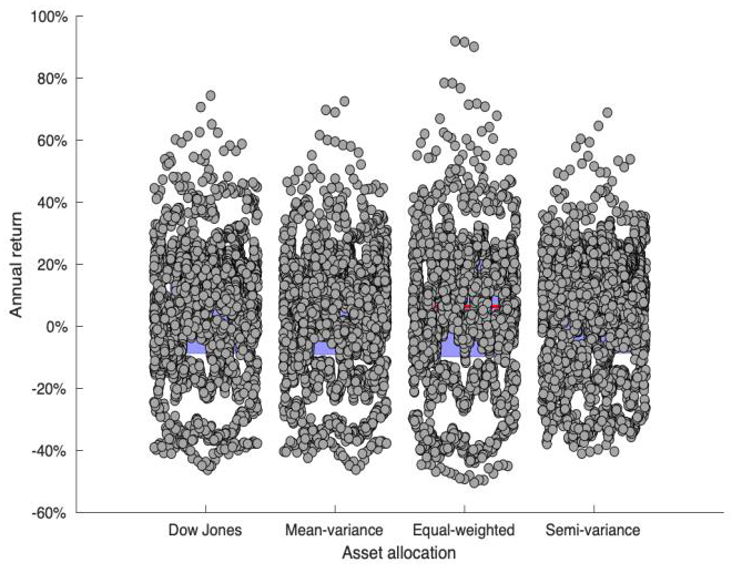
Source: own elaboration using Campbell (2021) and data from FactSet.
Figure 1 Data points visualization for annual returns (Jan 4, 1999 - May 29, 2020). Para Mean-variance Portfolio w≤0.05, Equal-weighted w=0.033, Semi-variance Portfolio w≤0.15.
The same conclusions are obtained when analyzing Figure 2, where the semi-variance strategy has a lower dispersion of annual returns between 2000-2020, among the four strategies analyzed.
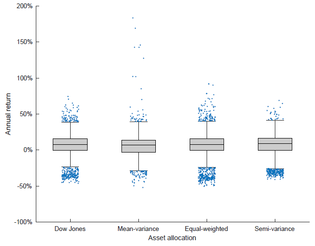
Source: own elaboration and data from FactSet.
Figure 2 Box plot for rolling annual returns (Jan 4, 1999 - May 29, 2020). Para Mean-variance Portfolio w≤0.05, Equal-weighted w=0.033, Semi-variance Portfolio w≤0.15.
To study the similarity of the strategies with respect to the strategy of holding the DJIA, histograms are calculated (see Figure 3). The Mean-variance strategy is the one with the highest number of observations with respect to the average returns. The other two strategies have similar annual return frequencies.
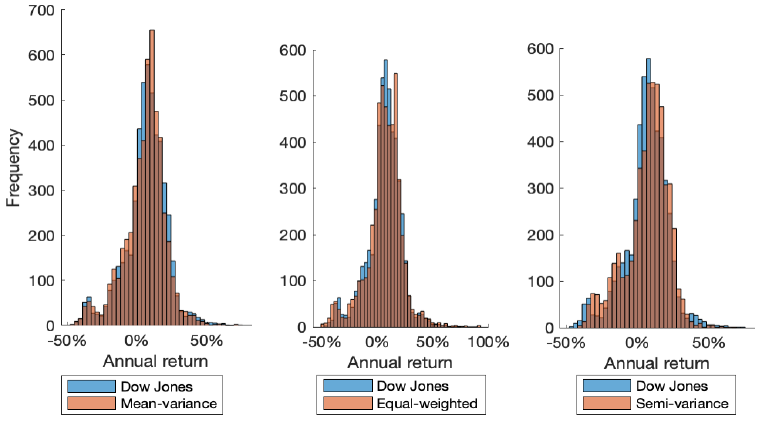
Source: own elaboration and data from FactSet.
Figure 3 Histograms for annual returns (2000-2020). Para Mean-variance Portfolio w≤0.05, Equal-weighted w=0.033, Semi-variance Portfolio w≤0.15.
Using different restrictions on the maximum percentage to invest in each asset. The Mean-variance strategy found a maximum probability of 44.9% in outperforming the DJIA one-year return (see Table 2). In none of the restrictions was a better risk-return ratio obtained (see Table 2, last two columns). For the Equal-weighted strategy, although it has a higher probability (51.1%) of outperforming the DJIA, its return-risk ratio is lower (see Table 3). On the other hand, for the semi-variance strategy with any type of restriction, the probability of outperforming the DJIA is between 60.2%-65.2%, with a better risk-return ratio for all restrictions (see Table 4).
Table 5 shows the performances (risk-adjusted) of the three strategies using the CAPM. Applying linear regression to solve equation (3). It is observed that the three alphas are significantly different from zero. And the models explain 94.6%, 97.22% and 87.58% in how the data vary. We conclude that the Mean-variance and Equal-weighted strategies do not outperform the market, having negative alphas. The Semi-variance strategy does outperform the market with an annual abnormal return of 0.42%. On the other hand, the strategy has a slightly lower risk than the market risk, as it has a beta (β) less than one.
To distinguish whether the strategy using the semi-variance is superior to the average of the mutual funds, taking a risk adjustment. Table 5 shows an appraisal of 1.34 for semi-variance strategy which is slightly higher than the average appraisal of the mutual funds in Table 6. In 5 years out of the 7 analyzed by Wang (2017).
Conclusion
It was found that portfolio optimization under semi-variance is more relevant than mean-variance optimization or by index investing. In the period analyzed and having the DJIA as a target, the best way to run a passive portfolio strategy was by optimizing the minimum semi-variance. The semi-variance is calculated with the yield spread below the annual return of the DJIA. The weights of the best portfolio are less than 15%. This strategy has a 65.2% probability of outperforming the DJIA annual return. 5 134 simulations are performed between 2000-2020. Obtaining an annual abnormal return of 0.42% and a beta of 0.95. Therefore, the proposal obtains a higher risk-adjusted return with a risk slightly lower than the risk of the DJIA.
This study leaves aside the investor's perception of risk. Although there is no consensus in the literature that semi-variance is related to portfolio risk perception. Veld & Veld-Merkoulova (2008) study the risk perceptions of individual investors and found that most investors use the semi-variance of returns as a measure of risk. While bond investors prefer the probability of loss. Market return being the most important benchmark. In contrast other authors found that optimization by semi-variance may not be appropriate for different risk profiles. Hoe et al. (2010) use four different portfolio optimization models that employ different risk measures: variance, absolute deviation, minimax, and semi-variance. With the minimax model is appropriate for investors who have a strong downside risk aversion. The perception of risk is left to future research.

