


 nueva página del texto (beta)
 Inglés (pdf)
 Artículo en XML
 Referencias del artículo
 Enviar artículo por email
 Citado por SciELO
  Similares en
SciELO
Similares en
SciELO 
 Permalink
Introduction
Keating & Shadwick (2002) propose the Omega ratio as a measure of the performance of investment strategies or portfolios. In addition to evaluating strategies or portfolios, it is used to assemble portfolios, under the assumption that past performance will influence future performance to a certain extent. Either for short-, medium- and long-term investment strategies or asset allocation (Gaspars-Wieloch & Michalska, 2016). In this paper the Omega ratio is used to asset allocation with a one-year investment horizon. Where the assets to be chosen are the components of the Dow Jones Industrial Average. These assets are invested for one year, even if there is a change in the index. Different criteria are used to asset allocation and the results are compared with the performance of the index and other strategies that use the upside-potential, downside-potential and semi-variance.
Empirical studies favoring the use of the Omega ratio. Bernard et al. (2019) showed that maximizing the Omega ratio with restrictions is a risky strategy and sometimes coincides with the choice made by risk-neutral investors. Georgantas et al. (2021) for the US market between 2005-2016 compare the Omega ratio with mean-variance and conditional value-at-risk (CVaR), where the Omega ratio is not among the best criteria to include for portfolio construction. Castro et al. (2021) study portfolios of real projects, proposing optimization through the maximization of Omega-ratio vs. Sharpe-ratio. Resulting in Omega-ratio being the best optimization.
This paper compares the omega ratio with the mean-variance, and instead of using CVaR, the downside-potential and the semi-variance are used for risk. The period of analysis is between 2000-2020, using rolling windows of annual returns of each day. We have a total of 5,134 observations for each index component, and thus obtain more robust results.
The use in the literature of the omega ratio is generally accompanied with other constraints within the optimization model. Sehgal & Mehra (2021) optimize portfolios using the Omega ratio, the semi-moderate absolute deviation ratio and the stable-tail adjusted return-weighted adjusted return ratio (STARR). They note that it is necessary to consider constraints in the optimization when the number of assets and scenarios is large. The assets used are those contained in the FTSE 100, Nikkei 225, S&P 500, and S&P BSE 500 indices. They conclude that the models used to improve the statistics measured by standard deviation, value at risk (VaR), conditional value at risk (CVaR), Sharpe ratio, and weighted stable tail adjusted return ratio (STARR). Other types of restrictions taken from the literature are also included in this paper. Although not only increasing the type of restrictions helps to improve the results. Gilli et al. (2008, 2011) includes an algorithm that generates different scenarios and includes short sales. By creating scenarios and using the Omega function, they detected portfolios with good results in terms of performance. They obtain better returns with higher volatility because Omega does not penalize asset variability. Mean-variance portfolios were compared, Omega with only long positions and Omega with short and long positions, the latter being the best portfolio. Sharma & Mehra (2017) propose an omega ratio optimization model in conjunction with mean-variance models. This way of optimizing the portfolio gives better results compared to models where only the omega ratio is used. Better results in relation to higher omega ratio. Omega-ratio is also used in conjunction with other metrics to optimize a portfolio. Taylor (2022) model expected shortfall (ES) as the product of VaR and a factor that is a function of a time-varying Omega ratio.
The Omega ratio is used in the same way for passive portfolio management as for active portfolio management. Gunning & Van (2020) use the volatility of the return spread (tracking error, i.e., portfolio return minus target return) to measure market conditions and to be able to restrict portfolio construction and include short sales in their strategy. Another use is the evaluation of portfolio performance for specific investor profiles. Acosta-Osorio (2018) finds that the Omega-ratio can be optimal alternative criteria for rating the performance of an investment profile. He classifies them as "unsatisfied risk-averse investors". There are a variety of ways to use Omega-ratio. Liesiö et al. (2021) analyzed 148 articles in which they found a wide range of different application domains and the use of multiple methodologies.
Although there are arguments for and against the use of the omega ratio to optimize portfolios, most of the literature does not compare this strategy against a passive portfolio strategy (index investing). Since the investor needs to know the probability of profit we would have against the index and the expected average return differential. And depending on the investor profile will make better decisions on the passive portfolio strategy.
Zhang, Y. et al. (2018) review the literature of 197 papers, and they find the main groupings of the studies in dynamic optimization, robust optimization, and fuzzy optimization. They mention that the difference in horizons should be considered, and normality assumptions are not real. In addition, investors want to know what is happening now, what is likely to happen next, and what steps should be taken to obtain optimal portfolios. To answer part of the findings of these authors we put forward the following hypothesis.
Postmodern portfolio theory better allocates economic resources to an investment portfolio compared to modern portfolio theory when the portfolio is dynamically optimized using a minimum variance. This is because the volatility used by the modern theory weights positive and negative movements equally to maintain a normal distribution (price increases/decreases), while the postmodern theory differentiates between positive and negative movements of the asset price, whose distribution is different from the normal one. The study is restricted to one-year investment periods and looks for the best performance.
Through the development of three sections: methodology, results, and conclusions. We seek to answer the question: Is the omega ratio (Ω) a good portfolio optimization criterion?
Methodology
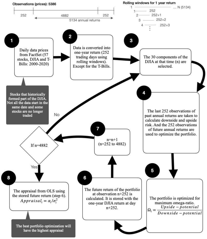
To increase the number of observations and thus obtain more robust results. Annual returns calculated by rolling window during each day between 2000-2020 are used. Since the objective is asset allocation and not security selection, it is limited to the choice between 30 assets contained in the Dow Jones Industrial average. In the study period the index has had 15 revisions (see Table 1) with a total of 48 different assets.
Table 1 Changes in the components of the Dow Jones Industrial Average: 2000-2020.
| 1 | 01/11/1999 | 6 | 08/06/2009 | 11 | 01/02/2018 |
| 2 | 08/04/2004 | 7 | 24/09/2012 | 12 | 26/06/2018 |
| 3 | 21/11/2005 | 8 | 23/09/2013 | 13 | 02/04/2019 |
| 4 | 19/02/2008 | 9 | 19/03/2015 | 14 | 06/04/2020 |
| 5 | 22/09/2008 | 10 | 01/09/2017 | 15 | 31/08/2020 |
Source: FactSet.
Initially, 4 portfolios are optimized, whose restrictions are the Upside-potential, Downside-potential, Semi-variance and Omega-ratio. For different investment maxima in each DJIA asset.
For the evaluation of portfolio performance using out-of-sample data, appraisal is used. Whose performance in the appraisal formula (equation 6) is measured by alpha. It does not mean that the higher the Alpha or the higher the risk-adjusted return, the better the portfolio. Since the abnormal return obtained may have been obtained with a higher specific risk than the rest of the portfolios. Treynor & Black (1973) propose the Appraisal to differentiate performance. Starting from the CAPM (equation 1) we can obtain the systematic risk, or risk that cannot be diversified. And the unsystematic risk, or specific risk, which is the variance of the error term of the CAPM. The Appraisal is obtained by dividing the Alpha by this variance (equation 6).
Based on the resulting ranges in the omega-ratio simulation, the constraint of the maximum to invest in each asset is taken and whether to simulate with different omega-ratio maxima.
Part of these ideas were taken from the article by Wagner & Uryasev (2019). They optimize portfolios using restrictions on the value of negative expectable and the omega ratio. Expectable are like quantiles, except that they are defined by the expectations of the probability distribution. In one of the models proposed in this paper we will use constraints on the value of the omega ratio to improve the optimization results (Omega-ratio < 470).
To select the best model among five, Appraisal is applied. See figure 1 for the methodology process. Details of the metric are given in the next section.
Results
Table 2 shows the simulation results, with restrictions between 5% to 100% of maximum investment in each of the 30 assets of the index, during the study period. The minimum downside-potential optimization is sought. It is compared with the investment in the DJIA. The probability of outperforming the index is close to 50% and the risk-return ratio of the DJIA is generally above the Downside-potential.
Table 2 Simulations results for the Downside-potential portfolios (2000-2020)
| Maximum percentage to be invested in each asset |
Probability of annual return > DJIA |
Average anual return DJIA |
Average annual return Downside- Portfolio |
Standard deviation DJIA |
Standard deviation Downside- Portfolio |
DJIA (Return / volatility) |
Downside (Return / volatility) |
|---|---|---|---|---|---|---|---|
| 5.0% | 60.7% | 6.3% | 6.6% | 14.9% | 15.0% | 0.42 | 0.44 |
| 10.0% | 62.6% | 6.3% | 7.2% | 14.9% | 14.5% | 0.42 | 0.50 |
| 15.0% | 61.7% | 6.3% | 6.5% | 14.9% | 14.5% | 0.42 | 0.45 |
| 20.0% | 60.8% | 6.3% | 6.4% | 14.9% | 14.9% | 0.42 | 0.43 |
| 25.0% | 56.8% | 6.3% | 6.4% | 14.9% | 15.1% | 0.42 | 0.42 |
| 30.0% | 53.4% | 6.3% | 6.1% | 14.9% | 15.1% | 0.42 | 0.40 |
| 35.0% | 49.8% | 6.3% | 5.9% | 14.9% | 15.4% | 0.42 | 0.38 |
| 40.0% | 50.5% | 6.3% | 5.7% | 14.9% | 15.6% | 0.42 | 0.37 |
| 45.0% | 50.0% | 6.3% | 5.6% | 14.9% | 16.1% | 0.42 | 0.35 |
| 50.0% | 50.8% | 6.3% | 5.5% | 14.9% | 16.8% | 0.42 | 0.33 |
| 55.0% | 49.9% | 6.3% | 5.5% | 14.9% | 16.7% | 0.42 | 0.33 |
| 60.0% | 49.2% | 6.3% | 5.5% | 14.9% | 16.7% | 0.42 | 0.33 |
| 65.0% | 48.5% | 6.3% | 5.4% | 14.9% | 16.8% | 0.42 | 0.32 |
| 70.0% | 48.9% | 6.3% | 5.4% | 14.9% | 17.0% | 0.42 | 0.32 |
| 75.0% | 48.4% | 6.3% | 5.4% | 14.9% | 17.3% | 0.42 | 0.31 |
| 80.0% | 47.9% | 6.3% | 5.4% | 14.9% | 17.7% | 0.42 | 0.30 |
| 85.0% | 48.8% | 6.3% | 5.4% | 14.9% | 18.2% | 0.42 | 0.30 |
| 90.0% | 50.0% | 6.3% | 5.4% | 14.9% | 18.7% | 0.42 | 0.29 |
| 95.0% | 50.9% | 6.3% | 5.3% | 14.9% | 19.3% | 0.42 | 0.28 |
| 100.0% | 59.4% | 6.3% | 10.2% | 14.9% | 20.1% | 0.42 | 0.51 |
Source: own elaboration and data from FactSet.
For the Upside-potential (see Table 3) the probabilities are greater than 50% in all cases, but at a higher cost in volatility.
Table 3 Simulations results for the Upside-potential portfolios (2000-2020)
| Maximum percentage to be invested in each asset |
Probability of annual return > DJIA |
Average anual return DJIA |
Average annual return Upside- Portfolio |
Standard deviation DJIA |
Standard deviation Upside- Portfolio |
DJIA (Return / volatility) |
Upside (Return / volatility) |
|---|---|---|---|---|---|---|---|
| 5.0% | 55.4% | 6.3% | 6.3% | 14.9% | 15.2% | 0.42 | 0.42 |
| 10.0% | 51.4% | 6.3% | 6.4% | 14.9% | 15.3% | 0.42 | 0.42 |
| 15.0% | 52.7% | 6.3% | 6.5% | 14.9% | 15.7% | 0.42 | 0.42 |
| 20.0% | 54.7% | 6.3% | 6.8% | 14.9% | 16.1% | 0.42 | 0.42 |
| 25.0% | 52.9% | 6.3% | 6.8% | 14.9% | 16.8% | 0.42 | 0.40 |
| 30.0% | 52.3% | 6.3% | 6.9% | 14.9% | 17.1% | 0.42 | 0.40 |
| 35.0% | 53.1% | 6.3% | 6.8% | 14.9% | 17.6% | 0.42 | 0.39 |
| 40.0% | 52.8% | 6.3% | 6.6% | 14.9% | 17.9% | 0.42 | 0.37 |
| 45.0% | 53.3% | 6.3% | 6.4% | 14.9% | 18.5% | 0.42 | 0.35 |
| 50.0% | 53.2% | 6.3% | 6.2% | 14.9% | 19.4% | 0.42 | 0.32 |
| 55.0% | 52.7% | 6.3% | 6.3% | 14.9% | 19.3% | 0.42 | 0.33 |
| 60.0% | 52.5% | 6.3% | 6.3% | 14.9% | 19.2% | 0.42 | 0.33 |
| 65.0% | 52.5% | 6.3% | 6.4% | 14.9% | 19.3% | 0.42 | 0.33 |
| 70.0% | 53.6% | 6.3% | 6.4% | 14.9% | 19.5% | 0.42 | 0.33 |
| 75.0% | 54.3% | 6.3% | 6.5% | 14.9% | 19.8% | 0.42 | 0.33 |
| 80.0% | 54.5% | 6.3% | 6.5% | 14.9% | 20.2% | 0.42 | 0.32 |
| 85.0% | 53.6% | 6.3% | 6.5% | 14.9% | 20.7% | 0.42 | 0.32 |
| 90.0% | 53.6% | 6.3% | 6.6% | 14.9% | 21.2% | 0.42 | 0.31 |
| 95.0% | 53.6% | 6.3% | 6.6% | 14.9% | 21.9% | 0.42 | 0.30 |
| 100.0% | 53.7% | 6.3% | 6.7% | 14.9% | 22.6% | 0.42 | 0.30 |
Source: own elaboration and data from FactSet.
In Table 4 where the omega-ratio is used, the probability of outperforming the DJIA is increased. The probability is 62.3% with a maximum investment of 10%-15% in each asset. The above with a lower volatility compared to the index.
Table 4 Simulations results for the Omega-ratio portfolios (2000-2020)
| Maximum percentage to be invested in each asset |
Probability of annual return > DJIA |
Average anual return DJIA |
Average annual return Omega- Portfolio |
Standard deviation DJIA |
Standard deviation Omega- Portfolio |
Max. Omega | Min. Omega |
|---|---|---|---|---|---|---|---|
| 5.0% | 60.5% | 6.3% | 6.5% | 14.9% | 15.1% | 26 | 2 |
| 10.0% | 62.3% | 6.3% | 7.2% | 14.9% | 14.4% | >470 | 6 |
| 15.0% | 62.3% | 6.3% | 6.7% | 14.9% | 14.6% | >470 | 11 |
| 20.0% | 61.9% | 6.3% | 6.8% | 14.9% | 15.1% | >470 | 7 |
| 25.0% | 59.1% | 6.3% | 7.0% | 14.9% | 15.3% | >470 | 20 |
| 30.0% | 57.2% | 6.3% | 7.2% | 14.9% | 15.6% | >470 | 27 |
| 35.0% | 54.5% | 6.3% | 7.4% | 14.9% | 16.1% | >470 | 36 |
| 40.0% | 54.7% | 6.3% | 7.4% | 14.9% | 16.4% | >470 | 46 |
| 45.0% | 54.6% | 6.3% | 7.6% | 14.9% | 16.8% | >470 | 61 |
| 50.0% | 55.8% | 6.3% | 7.7% | 14.9% | 17.3% | >470 | 84 |
| 55.0% | 55.3% | 6.3% | 7.7% | 14.9% | 17.4% | >470 | 96 |
| 60.0% | 55.2% | 6.3% | 7.7% | 14.9% | 17.5% | >470 | 111 |
| 65.0% | 54.6% | 6.3% | 7.8% | 14.9% | 17.5% | >470 | 130 |
| 70.0% | 54.5% | 6.3% | 7.8% | 14.9% | 17.5% | >470 | 136 |
| 75.0% | 54.3% | 6.3% | 7.8% | 14.9% | 17.6% | >470 | 142 |
| 80.0% | 54.1% | 6.3% | 7.8% | 14.9% | 17.7% | >470 | 146 |
| 85.0% | 54.1% | 6.3% | 7.8% | 14.9% | 17.8% | >470 | 152 |
| 90.0% | 54.1% | 6.3% | 7.8% | 14.9% | 17.8% | >470 | 161 |
| 95.0% | 54.4% | 6.3% | 7.9% | 14.9% | 17.9% | >470 | 182 |
| 100.0% | 54.6% | 6.3% | 7.9% | 14.9% | 18.1% | >470 | 213 |
Source: own elaboration and data from FactSet.
To improve the results, the restriction of an omega-ratio maximum is added, between 20 and 470. Excluding 20, the probability of outperforming the DJIA is improved, and the volatility level is kept below or equal.
Table 5 Simulations results for the Omega <470 portfolios (2000-2020)
| Optimization criterion |
|||||||
|---|---|---|---|---|---|---|---|
| Maximum percentage to be invested in each asset |
Probability of annual return > DJIA |
Average anual return DJIA |
Average annual return Omega- Portfolio |
Standard deviation DJIA |
Standard deviation Omega- Portfolio |
Max. Omega | Min. Omega |
| 15.0% | 62.2% | 6.3% | 7.0% | 14.9% | 14.6% | 20 | 4 |
| 15.0% | 63.7% | 6.3% | 7.0% | 14.9% | 14.7% | 70 | 4 |
| 15.0% | 63.4% | 6.3% | 7.0% | 14.9% | 14.7% | 120 | 4 |
| 15.0% | 64.0% | 6.3% | 7.0% | 14.9% | 14.8% | 170 | 4 |
| 15.0% | 63.9% | 6.3% | 7.0% | 14.9% | 14.8% | 220 | 4 |
| 15.0% | 64.0% | 6.3% | 7.0% | 14.9% | 14.8% | 270 | 4 |
| 15.0% | 63.8% | 6.3% | 7.0% | 14.9% | 14.8% | 320 | 4 |
| 15.0% | 63.6% | 6.3% | 7.0% | 14.9% | 14.9% | 370 | 4 |
| 15.0% | 63.8% | 6.3% | 6.9% | 14.9% | 14.9% | 420 | 4 |
| 15.0% | 63.6% | 6.3% | 6.9% | 14.9% | 14.8% | 470 | 4 |
Source: own elaboration and data from FactSet.
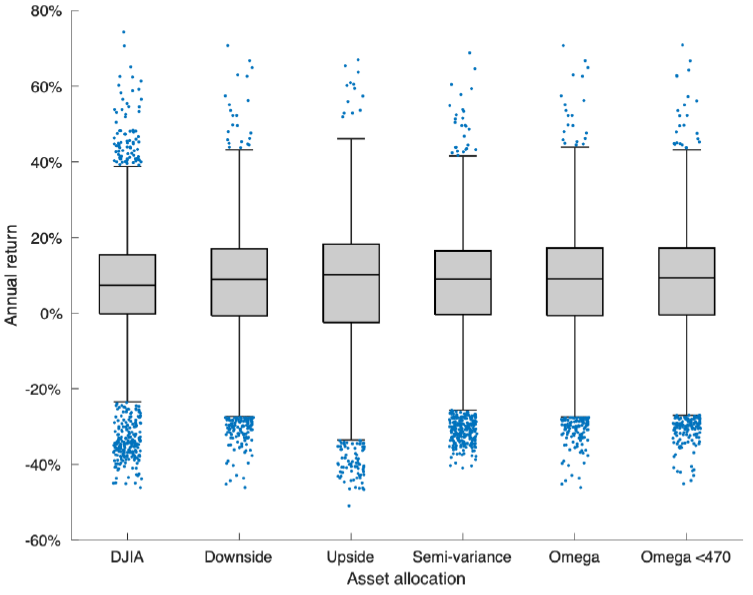
To differentiate the behaviors in the simulation of the 6 portfolios, the annual returns are visualized in Figure 1. Although it is easier to observe their maximum and minimum returns, it is not possible to compare them by their level of risk. Therefore, the CAPM (equation 3) is used to obtain the performance and level of risk with respect to the market (Alpha and Beta, respectively).
Table 6 shows that the 5 portfolios have a risk-adjusted performance greater than the market (Alpha greater than zero) with a significance level of 100%. In addition, all portfolios have a lower risk than the market (Beta less than 1).
Downside-potential w ≤ 0.15, Upside-potential w = 0.20, Semi-variance Portfolio w ≤ 0.15, Omega w ≤ 0.15, Omega < 0.15, & w ≤ 0.15.
Source: own elaboration and data from FactSet.
Figure 2 Rolling window annual returns (2000-2020).
Table 6 CAPM results for the portfolios (2000-2020).
| Estimate | Standard error | T-statistic | P-value | |
|---|---|---|---|---|
| Minimum downside-potential, weight for each asset <=15% Portfolio (R-squared 0.7592) | ||||
| Alpha | 0.0093 | 0.0011 | 8.5084 | 0.0000 |
| Beta | 0.8508 | 0.0067 | 127.2082 | 0.0000 |
| Maximum upside-potential, weight for each asset <=20% Portfolio (R-squared 0.7249) | ||||
| Alpha | 0.0089 | 0.0013 | 6.9292 | 0.0000 |
| Beta | 0.9191 | 0.0079 | 116.2836 | 0.0000 |
| Minimum semi-Variance, weight for each asset <=15% Portfolio (R-squared 0.8758) | ||||
| Alpha | 0.0042 | 0.0008 | 5.1968 | 0.0000 |
| Beta | 0.9532 | 0.0050 | 190.2328 | 0.0000 |
| Maximum omega-ratio, weight for each asset <=15% Portfolio (R-squared 0.7472) | ||||
| Alpha | 0.0105 | 0.0011 | 9.3398 | 0.0000 |
| Beta | 0.8522 | 0.0069 | 123.1554 | 0.0000 |
| Maximum omega-ratio <470, weight for each asset <=15% Portfolio (R-squared 0.7904) | ||||
| Alpha | 0.0122 | 0.0010 | 11.6912 | 0.0000 |
| Beta | 0.8887 | 0.0064 | 139.1256 | 0.0000 |
Alpha indicates the potential-adjusted abnormal return.
Source: own elaboration and data from FactSet.
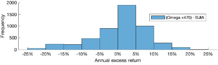
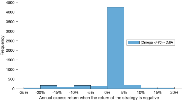
Calculating the Appraisal for the 5 portfolios (see Table 7), it is concluded that the best strategy is Omega-ratio (<470). Figure 3 shows the performance differential with respect to the DJIA, with a minimum of -25% and a maximum of 20%. Although, as mentioned above, if these portfolios are evaluated considering different degrees of risk, it is better to optimize using Omega-ratio. Figure 4 se. It shows the observations only when the return is negative (portfolios with omega-ratio), where there are mostly better observations than the DJIA (lower return drop).
Table 7 Appraisal ratio (2000-2020).
| Passive investments portfolios: optimization strategy | |||||
|---|---|---|---|---|---|
| Downside- potential |
Upside- potential |
Semi-variance | Omega-ratio | Omega-ratio (<470) |
|
| Appraisal | 1.64 | 1.13 | 1.34 | 1.74 | 2.36 |
Higher appraisal indicates better portfolio. Using 5,134 observations for each portfolio.
Source: own elaboration and data from FactSet.
Conclusions
In the period studied, the use of the Omega ratio as a measure to optimize portfolios does add value. This is observed in the appraisal, which uses the alpha based on a benchmark (DJIA) to compare portfolios with similar degrees of performance. The higher the appraisal, the greater the profit differential with respect to the risk assumed to obtain that differential. In addition, portfolios that use Omega for their optimization increase the probability of outperforming the DJIA (64%) with lower or equal volatility. To achieve this, it is necessary to include restrictions on the maximum investment in each asset (15%) and the maximum possible in the omega-ratio optimization (<470). Transaction costs have not been considered. When the strategy's return is negative, there is an 11.86% probability that it will underperform the DJIA during the study period. The results obtained cannot be compared with the literature, since they use different financial assets, different time periods, different investment horizons, or different ways of evaluating performance.
For future research, constraints can be added to the optimization to improve the results in this study. Sharma et al. (2017) use S&P 500 stocks to optimize portfolios whose return objectives depend on the distribution in the Omega ratio to control the conditional value-at-risk (CVaR). This optimization method maximizes the resulting Omega ratio in the simulation. They assume a loss-averse investor where the return objective depends on the CVaR at a confidence level (α), to reflect the investor's attitude towards losses.

