SciELO - Scientific Electronic Library Online

 
vol.67 número2Optimización del pago del IVA a través de un modelo de riesgo probabilístico para la planeación financiera índice de autoresíndice de materiabúsqueda de artículos
Home Pagelista alfabética de revistas  

Servicios Personalizados

Revista

Articulo

Indicadores

Links relacionados

  • No hay artículos similaresSimilares en SciELO

Compartir


Contaduría y administración

versión impresa ISSN 0186-1042

Contad. Adm vol.67 no.2 Ciudad de México abr./jun. 2022  Epub 10-Jul-2024

https://doi.org/10.22201/fca.24488410e.2022.3318 

Articles

Long memory in nominal exchange rates in Nigeria: An examination using fractionally integrated and cointegrated models with structural breaks

La larga memoria de los tipos de cambio nominales en Nigeria: un examen mediante modelos integrados fraccionalmente y cointegrados con rupturas estructurales

1 Monetary Programming Division, MPD, Central Bank of Nigeria, Nigeria

2 RR NGA, African Department, International Monetary Fund and MPC Secretariat Division, MPD, Central Bank of Nigeria, Nigeria

3 International Economic Relations Division, MPD, Central Bank of Nigeria, Nigeria.


Abstract

This study sets out to achieve two things majorly. First, is to scrutinize the performance of nominal exchange rates persistence in Nigeria, during the Pre-GFC and Post-GFC periods, in addition to using the full sample. The second is to ascertain whether, or not, the nominal exchange rates are fractionally cointegrated using the FCVAR model recently developed by Nielsen and Popiel (2018). The empirical results from the study depict higher exchange rates persistence in the post GFC period across all the currencies. The outcome lays credence to the need for stronger coordination between the fiscal and monetary authorities to adequately manage the exchange rates in the post-GFC period. We also find the presence of long-run properties in the Nominal exchange rates, where the CVAR is superior to the FCVAR for the full sample, and the FCVAR is superior to the CVAR for the Pre-GFC and Post-GFC periods, respectively.

JEL Code: C18; C51; F31; G15

Keywords: fractional integration; cointegrated VAR; exchange rates persistence; global financial crisis

Resumen

Este estudio se propone lograr dos cosas principalmente. La primera, es escudriñar el comportamiento de la persistencia de los tipos de cambio nominales en Nigeria, durante los periodos Pre- y Post-Crisis Financiera Mundial (CFM), además de utilizar la muestra completa. La segunda es determinar si, o no, los tipos de cambio nominales están fraccionalmente cointegrados utilizando el modelo FCVAR recientemente desarrollado por Nielsen y Popiel (2018). Los resultados empíricos del estudio muestran una mayor persistencia de los tipos de cambio en el período posterior a la CFM en todas las monedas. El resultado da crédito a la necesidad de una mayor coordinación entre las autoridades fiscales y monetarias para gestionar adecuadamente los tipos de cambio en el período posterior a la CFM. También encontramos la presencia de propiedades de largo plazo en los tipos de cambio nominales, donde el CVAR es superior al FCVAR para toda la muestra, y el FCVAR es superior al CVAR para los periodos Pre-CFM y Post-CFM, respectivamente.

Código JEL: C18; C51; F31; G15

Palabras clave: integración fraccional; VAR cointegrado; persistencia de los tipos de cambio; crisis financiera mundial

Introduction

After the pioneering works of Booth et al. (1982), Cheung (1993), and Baum et al. (1999), emphasis on the exchange rate shifted from conceptualization and pass-through to the understanding of its econometric characteristics. The exchange rate is a price that is very precious to the government. Its concept is sub-divided into two-the nominal and the real exchange rates.

The inquiry of exchange rate undercurrents and its cointegrating relationships has gained traction among researchers in the last three decades (see Baillie & Bollerslev, 1994a,b; Wang, 2004; Crato and Ray, 2000; and Fang et al. (1994). Studies on the exchange rates in Nigeria did not explicitly consider mean-reversion. Instead, they viewed the exchange rate as a macroeconomic variable and its impact on economic growth(see Oloyede and Fapetu, 2018; Ikpesu and Okpe, 2019) while others dwelled on its short-term forecasting(see Nyoni, 2018; Ejem and Ogbonna, 2019). Also, some studies considered its effect on the financial dollarization and remittance inflows (see Udoh and Udeaja, 2019; Adejumo and Ikhide, 2019).

The measurement of the degree of persistence is critical since it represents the stability of the country's Exchange rate. Furthermore, this type of information is useful for policymakers in the case of an exogenous shock, when alternative policy measures must be implemented based on the degree of persistence. Breaks in the series are another essential element of exchange rate data that must be modeled based on the data's particular properties. According to Taylor and Sarno (2001), research on the behavior of currency rates in transition economies is fairly scarce.

This study seeks to investigate the stochastic properties of exchange rates using the fractional cointegration VAR model with a multivariate set-up developed by Nielsen and Popiel (2018) and complemented with the univariate VAR model using weekly series. In line with the suggestions by Baillie & Bollerslev (1994a&b) and Diebold et al. (2004), persistence needs to be thoroughly investigated when dealing with cointegrating relationships of exchange rates. The need to enhance policy innovation and efficiency underscored the linkage of the observed shocks to the degree of persistence of exchange rates. Because of the relevance of the exchange rate to all facets of the Nigerian economy, including monetary policy decisions, and the fact that this study is the pioneering work on the test for the nominal exchange rates persistence in Nigeria pre and post the global financial crisis, necessitates the study.

Utilization of an alternative technique of Narayan et al. (2016) and Narayan and Liu (2015) GARCH-based approaches with different data frequencies (weekly and monthly) to test for the robustness in the nominal exchange rates. In contrast to other techniques applied in checking for robustness, the GARCH-based procedure is robust in handling data frequencies that are susceptible to elevated volatility.

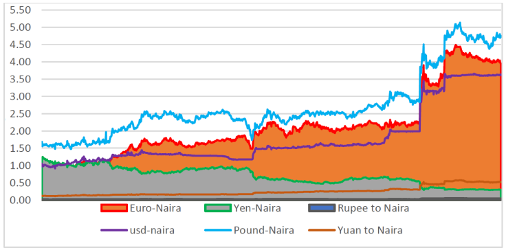
Finally, the descriptive statistics (see Table 1 Figure 1) clearly show an upward trend in the nominal exchange rates after the GFC, except in Yen-Naira, which is due to the continuous depreciation of the naira. This depreciation is further accounted for by Nigeria’s import-dependent economy and crude oil receipt of over 95% of government revenue and the attendant consequences on the purchasing power of the country. These remarkable distinctions in the behavioral pattern of the nominal exchange rates in Nigeria pre and post the global financial crisis generate a key excitement for empirically following the same path in the analyses

Table 1 Bai-Perron test for structural shift 

Exchange Rate Break date with intercept Break date With intercept and trend
USD 06/20/2005 06/20/2005
EURO 06/20/2005 06/20/2005
YEN 07/08/2002 07/08/2002
POUND 06/20/2005 07/15/2002
RUPEE 06/20/2005 06/20/2005
YUAN 06/20/2005 06/20/2005

From the results in Table 1 above, the absence of breaks Post-GFC period is confirmed, consequently, the data points are partitioned into the Pre- and Post-GFC periods.

Figure 1 Trend in Nominal Exchange Rates for selected currencies. 

Following the introduction, section 2 expounds on a review of the literature. The detailed methodology and data used are contained in section 3 whilst the empirical results are presented and discussed in section 4. Finally, Section 5 concludes the study.

Literature review

The literature on the dynamics of exchange rates could be categorized into two. They include the integer degrees of differentiation in exchange rate series (see Anthony and MacDonald,1999; Bleaney et al.,1999; Campa and Wolf, 1997 and Solis et al; 2002) and the long-run memory and fractional integration of exchange rates (see Booth et al., 1982; Cheung,1993; Baum et al.,1999; Crato and Ray, 2000; Gil-Alana and Mudida, 2018 and Wang, 2004).

Several studies have been conducted to investigate the existence or lack of long memory in exchange rates. Corazza and Malliaris (2002) conduct a study on foreign currency markets using the Hurst exponent and discover indications of long memory. Nath and Reddy (2002) examined the impact of long memory on the Indian foreign currency market versus the US dollar using Hurst R/S statistics and a variance ratio test. Peters (1996) investigated the Long Memory features of daily exchange rate data from the USD, Japanese yen, GBP, Euros, and Singapore dollar and discovered evidence of Long memory when utilizing the R/S technique. Bhar (1994) investigates Long memory in the Yen/dollar exchange rate and discovers no evidence of Long memory suggesting efficient pricing by market players when utilizing the modified R/S technique. kumar (2011) used the Hurst exponent, Hurst Mandelbrot R/S statistic, Lo's modified R/S statistic, Robinson's semi parametric estimator, and the modified GPH estimator to examine the presence of Long memory in the Indian foreign exchange market. The findings revealed that the Indian foreign currency market has a long memory.

Also, leveraging on data from 1980 to 2009, Arize (2011) showed the existence of a mean-reversion in both the linear and non-linear mean reversion for developing countries. Anouro et al. (2006) used a non-linear stationarity test to study the behavior of African exchange rates and uncovered that 11 out of the 13 are non-linear stationary. The result seems to suggest that bilateral nominal exchange rates are mean-reverting to the Purchasing Power Parity (PPP) equilibrium. Cashin and Mcdermott (2006) used data from 90 developed and developing countries. The outcome of the study shows that the speed of parity-reversion is slower for developing countries than developed countries, especially countries with fixed exchange rate regimes.

The effect of exchange rate shocks on the macroeconomy dominates the extant literature on the exchange rate for developing countries. For instance, Barhoumi (2007) using the structural VECM model, and the trends approach considers the exchange rate pass-through in 12 developing countries. The study concludes that the pass-through ratio in developing countries varies because of the diversity of structural shocks.

Lubinga and Kiiza (2013) applied a Panel-GARCH model to analyses the impact of the exchange rate dynamic bilateral trade flows between Uganda and her major trade partners. The evidence of the study suggests the importance of the issue of transitory or permanence of shocks in exchange rates for developing countries. Gil-Alana and Mudida (2018) examine nominal exchange rates in Kenya using the fractional integration technique. The evidence of the study suggests that exchange rates are nonstationary and non-mean-reverting

The empirical literature on exchange rates in Nigeria did not consider the issue of mean-reversion and, none of the existing studies either used the fractional integration approach or dichotomized the samples into pre-GFC and post-GFC. Also, none of the studies checked for robustness using the Garch-Model with weekly and monthly data frequencies. Most of the literature focuses mainly on using cointegration approaches to investigate the relationships between exchange rates and other macroeconomic variables. See (Ikpesu and Okpe (2019); Adejumo and Ikhide (2019); Oloyede and Fapetu (2018); Udoh and Udeaja (2019) and Nyoni (2018).

The literature on exchange rates in Nigeria mostly emphasizes the effect of exchange rate movement or regime on variables that determine the current behavior of the macro-economy. This study will contribute to the body of knowledge by filling the gap in the literature on the examination of shocks to nominal exchange rates in Nigeria to ascertain whether they are permanent or transitory using the fractional integration and fractional cointegration VAR models.

Methodology

The traditional univariate technique for evaluating persistence

A significant attribute of many time series data is non-stationarity. The evaluation of the persistence using the traditional univariate approach of order p [AR(p)] can be written as:

zt=α+γTrend+i=1pβizt-i+εt (1)

Given zt symbolizes the exchange rate, i=1pβi denotes the AR process, εtN0,σε2i.e. εt is I(0) and L is the lag operator Lzt=zt-1. Two potential situations for i=1pβi exist. If i=1pβi=0, subsequently zt has low persistence (or “short memory”) implying weak dependence of zt overtime. Hence, zt is I(0), i.e. zt is stationary at level. For policymaking, this scenario portends that actions taken by the central bank or monetary authority will not have a significant impact on exchange rates. Conversely, should i=1pβi>0, zt is understood to be highly persistent and exhibit long memory amongst observations. In this scenario, actions taken by the central bank or monetary authority will substantially affect the exchange rate. However, the Policy impact on exchange rates can either be temporary or permanent. The effect is temporary if zt 0<i=1pβi<1 while it is permanent if i=1pβi1. If the impact is temporary, it indicates that zt is mean reverting and the shocks will decay over a long horizon, However, if permanent, shocks will persist forever.

The fractionally integration model

The study also applies the fractional integration technique based on the recent findings in the literature (See Canarella and Miller, 2017; Gil-Alana and Carcel, 2018; Canarella and Miller, 2016; Usman and Akadiri, 2021 and Ebuh et al 2021) that stationary economic series can be given in a fractional form and may not take integer values. The fractional integration approach indicates that the series might be fractionally integrated. Such that shocks are not permanent but die out over long horizons.

Consequently, we examine Nigeria’s nominal exchange rates Zt using the fractionally integrated model to test for persistence:

1-LdZt=α+γTrend+εt; (2)

L is the lag operator LZt=Zt-1, d is any real number,  Zt is integrated of order d and symbolized by ZtId.εt is a covariance stationary process with a spectral density function that is positive and is an integrated order 0(I(0)) process and finite at zero frequency. Leveraging on the binomial expansion, 1-Ld polynomial in equation (2) can be formulated in such a way that for all real d,

1-Ld=j=0θjLj=j=0dj-1jLj=1-dL+dd-12L2-, (3)

Hence,

1-LdZt=Zt-dZt-1+dd-12Zt-2- (4)

Accordingly, Equation (1) is presented as follows:

Zt=α+γTrend+dZt-1+dd-12Zt-2-+εt (5)

Equation (5) is developed to emphasize the critical role d also plays in the calculation of the degree of persistence (Gil-Alana and Carcel, 2018). Three potential outcomes exist from using d to test for persistence. Suppose, if d=0, Zt (exchange rate) exhibits low-level persistence (i.e. “short memory”) also exchange rate is termed an I(0) series. If d falls within the interval of (0,0.5) is still supposed to exhibit long memory and is covariance stationary. However, suppose d0.5, this implies non-stationarity. Finally, suppose, 0.5 < d < 1 accordingly Zt is considered to be mean reverting and the effect of shocks to the exchange rate will disappear over in the long run. Nevertheless, suppose d1, it indicates policy shock will have a permanent influence.

We employ the parametric method in analyzing fractional integration which involves the maximum likelihood estimator of Sowell (1992). A major wrench to the fractional integration technique is the accuracy gained by leveraging on the news in the data via the parameter estimates. However, in line with Sowell (1992), a downside of the model is the sensitivity of the parameter estimates to models considered which could be misleading due to misspecification.

Fractionally cointegrated VAR (FCVAR) for nominal exchange rates

We examine Nigeria’s Nominal exchange rates, to check if they display long-run characteristics using the fractionally cointegrated VAR (FCVAR) proposed by Johansen (2008) and later extended by Johansen and Nielsen (2010, 2012), and Nielsen and Popiel (2018). The FCVAR allows for a fractional process of order d that cointegrates to order d-b. From a policy viewpoint, if Nominal exchange rates are cointegrated, this implies that policy targeted at one of the exchange rates will also influence other rates. Additionally, if the cointegration is fractional, the impact of policy on these rates will only disperse only after short horizons. Consider Zt as a vector of I(1) time series of the element p, the error correction form of the CVAR model is presented as follows:

ΔZt=αβ'Zt-1+i=1kΓiΔZt-i+εi=αβ'LZt+i=1kΓiΔLiZt+εt (6)

The FCVAR model is a derivative of Equation (6), this is done by interchanging the Δ and L with their fractional counterparts in Equation (7):

ΔdZt=αβ'Δd-bLbZt+i=1kΓiΔdLbiZt+εt, (7)

Given Δd is the term indicating fractional difference, and Lb=1-Δb is the fractional lag operator. Hence, α and β which are the long run parameters, p×r matrices were 0rp. The rank r is the cofractional rank. The columns of β comprise the r cofractional vectors such that β'Zt are the cointegrating combinations of the variables in the system. α represents the speed of adjustment towards equilibrium for each of the variables. Γ=Γ1,,Γk represents the short-run dynamics in the autoregressive process.(Nielsen and Popiel, 2018)2. Given that the CVAR is a unique case of the FCVAR, the FCVAR model condenses to the CVAR variant if. The FCVAR allows for simultaneous modeling of the short-run dynamics of the system, long-run equilibrium, and the correction to divergence from the equilibrium state.

The method of estimating the FCVAR follows the following steps: (a) the optimal lag length model is estimated; (b) the cointegration rank is established; (c) the data from (a) and (b) are employed to check for fractional cointegration; and in conclusion, (d) the Likelihood Ratio (LR) test is used to compare FCVAR model with the CVAR model by placing a limiting the null. If the null hypothesis is not accepted, then the FCVAR is favored, if not, the CVAR is accepted.

Results and discussions

Testing for structural shift in persistence

The Bai and Perron (2003) test is employed to test for structural shifts in persistence. The maximum number of structural breaks allowed in the time series is five. This procedure comprises a chronological application of test, assumed to produce an optimal result in selecting the number of breaks. The results are reported in Table 1

Preliminary analysis

Weekly data from 1999 to 2020 were used for the analyses. The nominal exchange rate pairings covered are USD-Naira, Euro-Naira, Yen-Naira, Pound-Naira, Rupee-Naira, and Yuan-Naira rates. The data for this study were sourced from the Central bank of Nigeria Statistical and Bloomberg databases. Various descriptive statistics carried out on the six nominal exchange rate variables were tabulated in Table 2. The data for the study were subdivided into two subsamples, given the results of the Bai-Perron test in Table 1 and consequently were split into Pre and post the Global financial crisis (GFC) individually. The Post-GFC captures the period of the crisis and afterward whilst the Pre-GFC is the period before September 2007. The Post-GFC stretch is so defined because of Nigeria’s peculiarity in which the effect of the GFC on macroeconomic fundamentals postdates the crisis period. Inferring from Table 2, the exchange rates for USD-Naira, Euro-Naira, Yen-Naira, Pound-Naira, Rupee-Naira, and Yuan-Naira exhibit higher volatility before the GFC than afterward.

Table 2 Descriptive statistics. 

Statistic Usd-Naira Euro-Naira Yen-Naira Pound-Naira Rupee to Naira Yuan to Naira
Full Sample
Mean 177.25 212.16 70.17 269.92 3.25 25.41
Standard Deviation 82.53 94.22 25.36 92.68 0.92 13.23
Skewness 1.45 1.13 -0.04 1.21 1.40 1.21
Kurtosis 0.58 0.39 -1.09 0.50 0.71 0.17
No. of Observations 1084 1084 1084 1084 1084 1084
Pre-GFC
Mean 122.53 137.21 94.92 207.26 2.70 14.99
Standard Deviation 12.10 30.18 11.26 37.55 0.29 1.59
Skewness -0.81 -0.22 0.30 -0.18 -0.21 -0.78
Kurtosis -0.58 -1.68 -0.77 -1.64 -1.42 0.77
No. of Observations 433 433 433 433 433 433
Post-GFC
Mean 213.52 261.88 53.76 311.51 3.62 32.32
Standard Deviation 89.05 89.19 17.60 94.92 1.00 13.01
Skewness 0.81 0.96 0.37 0.87 0.85 0.73
Kurtosis -1.08 -0.78 -0.27 -0.86 -0.92 -1.02
No. of Observations 652 652 652 652 652 652

Source: Authors’ Computation

Besides, the mean and standard deviations of the variables were higher Post-GFC than before GFC. Thus, implying the presence of more asymmetry GFC afterward on the nominal exchange rates.

The descriptive statistics and the plot of the six nominal exchange rate variables in Figure 1, clearly shows an upward trend in the nominal exchange rates after the GFC except in Yen-Naira. This upward trend in the nominal exchange rates could be attributed to the continuous depreciation of the naira. These outstanding distinctions in the behavioral pattern of the nominal exchange rates in Nigeria before and afterward of the GFC create the needed enthusiasm for empirically following the same path in the analyses.

Main results

The study examines the nominal exchange rates in Nigeria using the full, pre-GFC, and post-GFC sample periods to test for the existence and the degree of persistence of the nominal exchange rates in Nigeria. The study leveraged on the univariate and the fractional cointegrated VAR models with and without a trend. Table 3 presents the results on the traditional approach for persistence on the nominal exchange rates, which were observed to be non-stationarity as the magnitude of the persistence is close to unity for both with intercept and with intercept and trend. A further examination of the results shows that persistence is mean reverting in each sample considered, implying that the degree of persistence is temporal and not permanent. Thus, indicating that the nominal exchange rates will revert to their long-run mean.

Table 3 Traditional Approach with weekly Data 

Exchange Rate Full Sample Pre-GFC Post-GFC
Intercept Intercept and Trend Intercept Intercept and Trend Intercept Intercept and Trend
US i=1Pβi

  • 0.9995A

  • (0.0018)

  • 0.9970A

  • (0.0034)

  • 0.9871A

  • (0.0073)

  • 0.9662A

  • (0.0151)

  • 0.9991A

  • (0.0028)

  • 0.9932A

  • (0.0067)

i=1Pβi=1

  • 0.0515

  • [0.0019]

  • 0.6936

  • [0.0034]

  • 3.0638c

  • [0.0073]

  • 4.9853B

  • [0.0151]

  • 0.0827

  • [0.0028]

  • 0.9749

  • [0.0067]

Euro i=1Pβi

  • 0.9992A

  • (0.0018)

  • 0.9933

  • (0.0032)

  • 0.9964A

  • (0.0041)

  • 0.9832A

  • (0.0083)

  • 0.9981A

  • (0.0030)

  • 0.9901A

  • (0.0057)

i=1Pβi=1

  • 0.1735

  • [0.0018]

  • 4.15735B

  • [0.0032]

  • 0.7661

  • [0.0041]

  • 4.0311B

  • [0.0083]

  • 0.3824

  • [0.0030]

  • 2.5719

  • [0.0057]

Yen i=1Pβi

  • 0.9992A

  • (0.0021)

  • 0.9843A

  • (0.0061)

  • 0.9849A

  • (0.0092)

  • 0.9684A

  • (0.0133)

  • 0.9985A

  • (0.0030)

  • 0.9910A

  • (0.0054)

i=1Pβi=1

  • 0.1186

  • [0.0020]

  • 6.3971B

  • [0.0061]

  • 2.6348

  • [0.0091]

  • 5.5429B

  • [0.0133]

  • 0.2198

  • [0.0030]

  • 2.5368

  • [0.0054]

Pound i=1Pβi

  • 0.9991A

  • (0.0020)

  • 0.9916A

  • (0.0044)

  • 0.9939A

  • (0.0061)

  • 0.9582

  • (0.0145)

  • 0.9971A

  • (0.0034)

  • 0.9877A

  • (0.0074)

i=1Pβi=1

  • 0.1905

  • [0.0020]

  • 3.6047C

  • [0.0044]

  • 0.9661

  • [0.0061]

  • 8.2380A

  • [0.0145]

  • 0.4577

  • [0.0034]

  • 2.7425C

  • [0.0074]

Rupee i=1Pβi

  • 0.9983A

  • (0.0021)

  • 0.9940A

  • (0.0032)

  • 0.9921A

  • (0.0072)

  • 0.9522A

  • (0.0163)

  • 0.9971A

  • (0.0034)

  • 0.9925A

  • (0.0052)

i=1Pβi=1

  • 0.5944

  • [0.0021]

  • 3.3135B

  • [0.0032]

  • 1.19260

  • [0.0072]

  • 8.8508

  • [0.0160]

  • 0.6892

  • [0.0034]

  • 1.9915

  • [0.0052]

Yuan i=1Pβi

  • 0.9995A

  • (0.0015)

  • 0.9958A

  • (0.0036)

  • 0.9902A

  • (0.0607)

  • 0.9451A

  • (0.0165)

  • 0.9991A

  • (0.0480)

  • 0.9905A

  • (0.00723)

i=1Pβi=1

  • 0.0750

  • [11.5899]

  • 1.3061A

  • [0.0365]

  • 1.7989

  • [0.0730]

  • 11.0116

  • [0.0168]

  • 0.13559

  • [0.0026]

  • 1.7087

  • [0.0072]

(where () are standard errors, [] are p=values and A, B, C represent statistical significance at 1%, 5% and 10% respectively)

Also, the Wald test was used to if the degree of persistence is not statistically different from one. The outcome revealed that the persistence’s were statistically insignificant in all the samples at various degrees, except the US dollar exchange rate in the pre-GFC period.

Also, we compute the half-life estimates for a shock to Nigeria’s Nominal exchange rates. The half-life fundamentally reveals the period it takes for the impact of a shock on the exchange rates to divide into two. From the results presented in Table 4, it lends credence to the findings in the traditional approach that exchange rate persistence is higher in the post-GFC period than the pre-GFC period. This finding emphasizes the need for better coordination between the fiscal and the monetary authorities, to adequately manage the exchange rates in the post-GFC period.

Table 4 Half-Life of Nominal Exchange Rate in Nigeria 

Exchange Rate Pre-GFC Post-GFC
Intercept Intercept & Trend Intercept Intercept & Trend
USD 85.178 30.8151 835.521 110.543
EURO 203.308 43.508 404.751 80.418
YEN 65.614 28.892 602.164 85.947
POUND 168.194 21.675 276.657 72.508
RUPEE 87.688 18.348 250.963 98.112
YUAN 113.766 16.996 720.019 68.920

Note: If mean reverting, (i=1pβi<1), half-life is calculated as log0.5logi=1pβi.

To complement the traditional approach, we use a fractionally integrated approach to test for persistence. From Table 5, the estimates obtained using the fractionally integrated approach were reported under two cases (with intercept and with intercept and trend) and three samples (full sample, Pre-GFC, and Post-GFC), as with the traditional approach. Several features are noticeable in Table 1. First, all the estimated values are below 0.5, showing that the six nominal exchange rates under consideration are fractionally integrated and exhibit long memory. As in the traditional approach, we also find the level of persistence to be higher for the post-GFC sample for all exchange rates than the pre-GFC sample. Leveraging on the Wald test, the values of the fractional parameter estimates were statistically less than one, contrary to the traditional approach. This result indicates that, although the Nominal exchange rates exhibit long-run memory impact of any policy shock on the exchange rate to die out, it may not be permanent.

Table 5 Fractional Integration approach with weekly data 

Exchange Rate Full Sample Pre-GFC Post-GFC
Intercept Intercept and Trend Intercept Intercept and Trend Intercept Intercept and Trend
US d

  • 0.4998A

  • (0.00317)

  • 0.4998A

  • (0.0245)

  • 0.4993A

  • (0.0038)

  • 0.4988A

  • (0.0023)

  • 0.4997A

  • (0.0080)

  • 0.4996A

  • (0.0058)

d=1.0

  • -157.3953A

  • [0.0031]

  • -203.9144A

  • [0.0024]

  • -129.5156A

  • [0.0038]

  • -212.1853A

  • [0.0023]

  • -62.3133A

  • [0.0080]

  • -87.8942A

  • [0.0058]

Euro d

  • 0.4998A

  • (0.0038)

  • 0.4997A

  • (0.0026)

  • 0.4995A

  • (0.0030)

  • 0.4992A

  • (0.0049)

  • 0.4997A

  • (0.0065)

  • 0.4996A

  • (0.0045)

d=1.0

  • -130.5850A

  • [0.0038]

  • -185.3688A

  • [0.0026]

  • -165.3615A

  • [0.0030]

  • -101.8578A

  • [0.0049]

  • -76.8136A

  • [0.0065]

  • -109.7214A

  • [0.0045]

Yen d

  • 0.4998A

  • (0.0237)

  • 0.4997A

  • (0.0001)

  • 0.4992A

  • (0.0051)

  • 0.4990A

  • (0.0035)

  • 0.4997A

  • (0.0055)

  • 0.4996A

  • (0.0020)

d=1.0

  • -211.2268A

  • [0.0023]

  • -615.4258A

  • [0.0000]

  • -97.3192A

  • [0.0051]

  • -139.4428A

  • [0.0035]

  • -90.5102A

  • [0.0055]

  • -243.4207A

  • [0.0020]

Pound d

  • 0.4998A

  • (0.0034)

  • 0.4997A

  • (0.0021)

  • 0.4994A

  • (0.0045)

  • 0.4988A

  • (0.0054)

  • 0.4997A

  • (0.0047)

  • 0.4995A

  • (0.0074)

d=1.0

  • -146.1007A

  • [0.0034]

  • -233.3078A

  • [0.0021]

  • -109.0422A

  • [0.0027]

  • -91.2656A

  • [0.0054]

  • -106.1856A

  • [0.0047]

  • -67.0876A

  • [0.0074]

Rupee d

  • 0.4998A

  • (0.0022)

  • 0.4997A

  • (0.0014)

  • 0.4993A

  • (0.0027)

  • 0.4987A

  • (0.0046)

  • 0.4997A

  • (0.0042)

  • 0.4996A

  • (0.0052)

d=1.0

  • -217.6329A

  • [0.0022]

  • -338.4302A

  • [0.0014]

  • -184.1283A

  • [0.0027]

  • -108.6300A

  • [0.0046]

  • -117.3627A

  • [0.0042]

  • -95.9017A

  • [0.0052]

Yen d

  • 0.4998A

  • (0.0337)

  • 0.4998A

  • (0.0031)

  • 0.4993A

  • (0.0039)

  • 0.4984A

  • (0.0038)

  • 0.4997A

  • (0.0077)

  • 0.4996A

  • (0.0055)

d=1.0

  • -131.6817A

  • [0.0037]

  • -160.2069A

  • [0.0031]

  • -126.1796A

  • [0.0000]

  • -130.9244A

  • [0.0038]

  • -64.2660A

  • [0.0077]

  • -89.9208A

  • [0.0000]

(where () are standard errors, [] are p=values and A, B, C represent statistical significance at 1%, 5% and 10% respectively).

Are nominal exchange rates fractionally cointegrated in Nigeria?

In furtherance to the objective of the study, we evaluate the likelihood of fractional cointegration amongst the various nominal exchange rates. The test for fractional cointegration is because currencies from Nigeria’s major trading partners and its reserves expose the Nigerian economy to both commodity price and trade shock. Also, Nigeria’s economy largely depends on import and trade interconnectedness, which could impact on policy actions aimed at stabilizing the exchange rate. Thus, the six nominal exchange rate variables were tested for cointegration. The study estimated the FCVAR, which is a unique variant of the CVAR with a fractional value of the order of integration. This result is achieved by first obtaining the maximum lag value, followed by the rank. These two parameters are used to obtain the order of integration. Inferring from the results in Table 6, we observe across the three sub-samples, four cointegrating relationships for the full sample and five for the Pre-GFC and Post-GFC samples, respectively. This result implies the existence of a long-run relationship amongst the nominal exchange rates of the six selected currencies with Naira. For the full sample, cointegrating relationships are better formed using the CVAR model than the FCVAR as the estimated fractional parameter is greater than 1. However, in the two sub-samples, cointegrating relationships are better formed using the FCVAR model, as the fractional parameters are both 0.010. Hence, justifying the implementation of the fractional framework. Additionally, in Table 7, we find the data to lends support to estimating the fractional parameter using FCVAR over the conventional CVAR, for the sub-samples samples, as shown by the statistically significant LR statistics. However, the CVAR model is suitable to ascertain cointegrating relationships for the full sample period.

Table 6 FCVAR (Weekly) 

Rank Lag d
Full Sample 4 2 1.071(0.016)
Pre-GFC 5 3 0.010(0.000)
Post-GFC 5 3 0.010(0.000)

where: d represents the fractional parameter. The AIC is used in determining the optimal lag length. using, a maximum of lag 3. The Values of the standard errors of the Fractional parameter are presented in ( ).

Table 7 CVAR vs FCVAR (Weekly)3  

LR P-value
Full Sample 1.767 0.145
Pre-GFC 180.944 0.000
Post-GFC 102.708 0.000

Note: The LR test restricts the fractional parameter to 1 under the null hypothesis. A failure to reject the null implies the acceptance of the CVAR, while the opposite favour the FCVAR.

Robustness

We employed Narayan and Liu (2015) and Narayan et al. (2016) GARCH-based unit root techniques to check for the robustness of results. The benefit of using this approach over others, is its usefulness in allowing the error term to follow a GARCH based process, as against other methods. Tule et al. (2020), Salisu et al. (2020), Salisu and Adeleke (2016), Narayan and Liu (2015), and Narayan and Sharma (2015), argue the choice of data frequency is of importance in empirical analyses. On this note, we considered, in addition to the weekly series, a monthly data frequency of nominal exchange rates to supplement the results obtained.

The results were similar to the traditional approach and the fractionally integrated approaches (Table 8 & 9) with higher degrees of persistence observed in the post-GFC period. Also, from the FCVAR estimates (Table 10 & 11), using the monthly samples, we find similar results to the weekly frequency. The results from the CVAR are superior to the FCVAR for the full sample, and the FCVAR results are superior for the Pre-GFC and Post-GFC periods, respectively. From these findings, the results are unaffected by the different data frequencies.

Table 8  Narayan and Liu (2015) and Narayan et al. (2016) GARCH-based model (Monthly) 

Exchange Rate Full Sample Pre-GFC Post-GFC
Intercept Intercept and Trend Intercept Intercept and Trend Intercept Intercept and Trend
US i=1Pβi

  • 0.4679A

  • (0.0154)

  • 0.4996A

  • (0.0264)

  • 0.6675A

  • (0.0370)

  • 0.4762B

  • (0.1338)

  • 0.5655

  • (0.4908)

  • 0.3522A

  • (0.0376)

i=1Pβi=1

  • 1.7542

  • [0.1410]

  • 0.5094A

  • [0.6859]

  • 5.6500

  • [0.2222]

  • 0.7366

  • [0.2690]

  • 0.8333

  • [0.4823]

  • 0.0062

  • [6.5103]

Euro i=1Pβi

  • 0.7625A

  • (0.0424)

  • 0.5640A

  • (0.3325)

  • 0.7592A

  • (0.1107)

  • 0.7386A

  • (0.1300)

  • 0.7606A

  • (0.0061)

  • 0.7578A

  • (0.0626)

i=1Pβi=1

  • 8.0770

  • [0.0262]

  • 1.7504A

  • [0.0334]

  • 2.4554

  • [0.0085]

  • 4.0235

  • [0.1310]

  • 9.6458A

  • [0.0356]

  • 14.9652A

  • [0.0624]

Yen i=1Pβi

  • 0.8631A

  • (0.0178)

  • 0.7824A

  • (0.0405)

  • 0.9476

  • (0.0186)

  • 0.5278B

  • (0.2512)

  • 0.8221A

  • (0.0287)

  • 0.7594A

  • (0.0059)

i=1Pβi=1

  • 2.1831A

  • [0.0149]

  • 28.8481A

  • [0.0405]

  • 3.1102c

  • [0.0073]

  • 3.6732c

  • [0.2541]

  • 1.1494

  • [0.0243]

  • 16.1316A

  • [0.0059]

Pound i=1Pβi

  • 0.7522A

  • (0.0396)

  • 0.7373A

  • (0.0043)

  • 0.0590

  • (0.1442)

  • 1.0490A

  • (0.0001)

  • 0.8358A

  • (0.0339)

  • 0.8191A

  • (0.0385)

i=1Pβi=1

  • 6.7144 B

  • [0.0257]

  • 36.8985A

  • [0.0430]

  • 20.1432A

  • [0.1535]

  • 24.4638

  • [0.0020]

  • 1.8799

  • [0.0205]

  • 21.6258A

  • [0.0385]

Rupee i=1Pβi

  • 0.8915A

  • (0.0986)

  • 0.6000A

  • (0.1633)

  • 0.5286A

  • (0.0970)

  • 0.6000C

  • (0.3389)

  • 0.5286A

  • (0.0970)

  • 0.6951A

  • (0.0660)

i=1Pβi=1

  • 1.1674

  • [0.0764]

  • 5.9974B

  • [0.1633]

  • 0.4249A

  • [0.2050]

  • 0.20878

  • [0.8234]

  • 0.4249A

  • [0.2050]

  • 21.2741

  • [0.0660]

Yuan i=1Pβi

  • 0.5820A

  • (0.0337)

  • 0.5823A

  • (0.0336)

  • 0.3750A

  • (0.0607)

  • 0.2283A

  • (0.0881)

  • 0.6153A

  • (0.0480)

  • 0.5166

  • (0.0633)

i=1Pβi=1

  • 0.1726

  • [11.5899]

  • 153.8729A

  • [0.0033]

  • 3.3252

  • [0.1004]

  • 76.6110

  • [0.0764]

  • 0.7208A

  • [1.4948]

  • 58.2120B

  • [0.0633]

where () are standard errors, [] are p=values and A, B, C represent statistical significance at 1%, 5% and 10% respectively).

Table 9  Narayan and Liu (2015) and Narayan et al. (2016) GARCH-based model (Monthly) 

Exchange Rate Full Sample Pre-GFC Post-GFC
Intercept Intercept and Trend Intercept Intercept and Trend Intercept Intercept and Trend
US i=1Pβi

  • 0.1638A

  • (0.0452)

  • 0.1605B

  • (0.0453)

  • 0.4675A

  • (0.1290)

  • 0.4491B

  • (0.1772)

  • 0.5971

  • [0.3872]

  • 1.1663

  • [0.4204]

i=1Pβi=1

  • 0.0008

  • [0.0030]

  • 0.1762

  • [3.6442]

  • 0.1695

  • [3.4156]

  • 8.5846

  • [0.0043]

  • 0.2285

  • (0.2172)

  • 0.5752 C

  • (0.2992)

Euro i=1Pβi

  • 0.8130A

  • (0.0786)

  • 0.7784

  • (0.1011)

  • 0.8560A

  • (0.1649)

  • 1.0453A

  • (0.0003)

  • 0.7671

  • (0.1247)

  • 0.7567A

  • (0.1377)

i=1Pβi=1

  • 2.6551

  • [0.0504]

  • 5.0639B

  • [0.0885]

  • 0.3702

  • [0.0091]

  • 23.9459A

  • [0.0058]

  • 0.5682

  • [0.1113]

  • 2.3352

  • [0.1417]

Yen i=1Pβi

  • 0.3794

  • (0.2175)

  • 0.3104

  • (0.4088)

  • 0.2310 B

  • (0.0496)

  • 0.3104

  • (0.4088)

  • 0.7896A

  • [0.1113]

  • 0.7872A

  • (0.1193)

i=1Pβi=1

  • 0.0044A

  • [0.7242]

  • 0.4296

  • [0,4506]

  • 0.6321

  • [0.6029]

  • 0.4296

  • [0.4506]

  • 2.90714C

  • (0.0739)

  • 3.1762B

  • [0.1193]

Pound i=1Pβi

  • 0.8686

  • (0.0548)

  • 0.8591

  • (0.0669)

  • 0.8266A

  • (0.1023)

  • 1.0493A

  • (0.0003)

  • 0.6165B

  • [0.2395]

  • 0.5743B

  • (0.2719)

i=1Pβi=1

  • 1.7816

  • [0.0353]

  • 5.4031

  • [0.0577]

  • 0.4496

  • [0.0533]

  • 1.3582

  • [0.0124]

  • 0.3118

  • (0.2377)

  • 0.5684

  • [0.2588]

Rupee i=1Pβi

  • 0.4284

  • (0.2912)

  • 0.4087

  • (0.3247)

  • 0.8437B

  • (0.2409)

  • 1.0612A

  • (0.0002)

  • 0.4389

  • [0.3529]

  • 0.4429

  • (0.3445)

i=1Pβi=1

  • 3.0261C

  • [0.2340]

  • 3.3136C

  • [0.3247]

  • 0.3538

  • [0.1930]

  • 42554.12A

  • [0.0002]

  • 1.1301

  • (0.2894)

  • 2.6140

  • [0.3445]

Yuan i=1Pβi

  • 0.7145A

  • (0.0593)

  • 0.6984A

  • (0.0625)

  • 0.5353A

  • (0.1347)

  • 0.6493

  • (0.9447)

  • 0.9313A

  • (0.0298)

  • 1.0367

  • (0.1450)

i=1Pβi=1

  • 0.0018

  • [0.1771]

  • 0.0496

  • [1.2478]

  • 0.0034

  • [169.3007]

  • 0.1378

  • [0.9468]

  • 0.1234

  • [0.2520]

  • 0.0005

  • [69.063]

(where () are standard errors, [] are p=values and A, B, C represent statistical significance at 1%, 5% and 10% respectively).

Table 10 FCVAR (Monthly) 

Rank Lag d
Full Sample 5 3 0.905 (0.049)
Pre-GFC 4 3 0.010 (0.000)
Post-GFC 4 3 0.010 (0.000)

where: d represents the fractional parameter. The AIC is used in determining the optimal lag length. using, a maximum of lag 3. The Values of the standard errors of the Fractional parameter are presented in ( ) .

Table 11 CVAR vs FCVAR. (Monthly) 

LR P-value:
Full Sample 3.037 0.181
Pre-GFC 216.485 0.000
Post-GFC 152.191 0.000

Note: under the null hypothesis, the LR test restricts the fractional parameter to 1. A failure to reject the null implies the acceptance of the CVAR, whilst the opposite favors the FCVAR.

Conclusions

This study sets out to achieve two key objectives. First, to examine the behavior of the nominal exchange rates persistence in Nigeria, during the Pre-GFC and Post-GFC periods, in addition to the full sample. Second, to ascertain whether or not, the nominal exchange rates are fractionally integrated. Consequently, for the main analysis, we adopt the traditional, fractionally integrated, and the fractionally cointegrated VAR models to analyze, the weekly frequency of the USD-Naira, Euro-Naira, Yen-Naira, Pound-Naira, Rupee-Naira, and Yuan-Naira nominal exchange rate variables.

We find, using both the traditional and fractionally integrated approaches, that the Post-GFC consistently maintains higher magnitudes of persistence for all exchange rates, than the Pre-GFC period. Both results suggest that the response of the nominal exchange rates to shocks were slower during the post-GFC than the Pre-GFC period. The result indicates the need for better coordination between the fiscal and monetary authorities, for the effective and efficient management of the exchange rates in the post-GFC era. Also, our results depict the nominal exchange rates, are fractionally cointegrated. The results, further reveal the FCVAR to be better in forming cointegrating relationships than the conventional CVAR for the Pre and Post-GFC periods. However, the reverse is the case, for the full sample results. The insight into this study is to aid policy innovation on exchange rates.

What are the most important takeaways from our findings? To begin, it is obvious that substantial policy actions must be adopted in the case of a shock in order to return the series to their original patterns. Second, for the series to respond more quickly, a proactive foreign exchange policy attitude is essential. Finally, this study may be expanded in numerous ways. Nonlinear structures may be considered in the context of fractional integration; moreover, the structural break technique used in this study can be expanded to allow for more flexible specifications, such as regime-switching models or time varying models.

References

Adejumo, A.O. and Ikhide, S.I. (2019). "The Effects of Remittance Inflows on Exchange Rates in Nigeria," Journal of Developing Areas, Tennessee State University, College of Business, vol. 53(1), pp.1-15, January-M [ Links ]

Anouro, E., Liew, V.K., and Elike, U. (2006), “Non-Linear Exchange Rate Behaviour: Are African Currencies Exceptional?” International Research Journal of Finance and Economics, Issue 1, 2006. [ Links ]

Anthony, M. and MacDonald, R. (1999). The width of the band and exchange rate mean reversion: some further ERM-based results, Journal of International Money and Finance vol.18, pp. 411-428. [ Links ]

Arize, A.C. (2011) “Mean Reversion in Real Exchange Rates in Seventy LDCs: An Empirical Investigation, International Journal- of Economics and Finance, Vol. 3, No. 5, October 2011. [ Links ]

Bai, Jushan, and Pierre Perron (2003), "Computation and analysis of multiple structural change models." Journal of applied econometrics 18.1 (2003): 1-22. [ Links ]

Baillie, Richard T., and Tim Bollerslev. "Cointegration, fractional cointegration, and exchange rate dynamics." The Journal of Finance 49.2 (1994a): 737-745. [ Links ]

Baillie, Richard T., and Tim Bollerslev. "The long memory of the forward premium." Journal of International Money and Finance 13.5 (1994b): 565-571 [ Links ]

Barhoumi, K. (2006): Exchange Rate Pass-Through and Structural Macroeconomic Shocks in Developing Countries: An Empirical Investigation. Available at https://mpra.ub.unimuenchen.de/6573/1/MPRA_paper_6573.pdfLinks ]

Baum, C.F., Barkoulas, J., Caglayan, M. (1999). Persistence in the international inflation rates. Southern Economic Journal vol.65, pp.900-913. [ Links ]

Bhar, R. (1994). Testing for long-term memory in yen/dollar exchange rate. Financial Engineering and the Japanese Markets, 1(2), 101-109. [ Links ]

Bleaney, M.F, Leybourne, S.J. and Mizen, P. (1999). Mean Reversion of Real Exchange Rates in High-inflation countries. Southern Economic Journal vol.65, pp.839. [ Links ]

Bloomberg, L.P. (2020) Nominal exchnage rate. Retrieved Feb. 8, 2020 from Bloomberg database. [ Links ]

Booth, G.G., Kaen, F.R., Koveos, P.E. (1982). R/S analysis of foreign exchange markets under two international monetary regimes. Journal of Monetary Economics vo.10, pp.407-415. [ Links ]

Campa, J.M., and Wolf, H. C. (1997). Is Real Exchange Rate Mean Reversion Caused by Arbitrage?, NBER Working Paper No. 6162. [ Links ]

Canarella, Giorgio, and Stephen M. Miller (2016), "Inflation persistence and structural breaks." Journal of Economic Studies. [ Links ]

Canarella, Giorgio, and Stephen M. Miller (2017), "Inflation targeting and inflation persistence: New evidence from fractional integration and cointegration." Journal of Economics and Business 92: 45-62. [ Links ]

Cashin, P. and McDermott, J.C (2006). "Parity Reversion in Real Exchange Rates: Fast, Slow, or Not at All?," IMF Staff Papers, Palgrave Macmillan, vol. 53(1), pp. 1-5. [ Links ]

Cheung, Y.W. (1993). Long memory in foreign exchange rates. Journal of Business and Economic Statistics vol.11, pp.93-101. [ Links ]

Chia, Cheng and Li (2012), “Exogenous Shocks and Exchange Rate Regimes” The World Economy, Vol. 35, Issue 4, pp. 444-460. [ Links ]

Corazza, M., & Malliaris, A. T. G. (2002). Multi-fractality in foreign currency markets. Multinational Finance Journal, 6(2), 65-98. [ Links ]

Crato, N. and Ray, B.K. (2000). Memory in returns and volatilities of future’s contracts. Journal of Futures Markets 20, pp.525-543. [ Links ]

Diebold, Francis X., Javier Gardeazabal, and Kamil Yilmaz. "On cointegration and exchange rate dynamics." The Journal of Finance 49.2 (1994): 727-735. [ Links ]

Dumrongrittkul, T. and Anderson, H.M. (2016), How Do Shocks to Domestic Factors Affect Real Exchange Rates of Asian Developing Countries?, Journal of Development Economics, Vol. 119, pp. 67-85. [ Links ]

Ebuh, G. U., Salisu, A., Oboh, V., & Usman, N. (2021). A test for the contributions of urban and rural inflation to inflation persistence in Nigeria. Macroeconomics and Finance in Emerging Market Economies, 1-25. [ Links ]

Ejem, C.A. and Ogbonna, U.G. (2019). "Modeling Volatility and Daily Exchange Rate Movement in Nigeria," International Journal of Economics and Financial Research, Academic Research Publishing Group, vol. 5(11), pp. 264-275. [ Links ]

Gil-Alana, L. and Mudida, R. (2018) Nominal Exchange Rates in Kenya. Are Shocks Transitory or Permanent? An Empirical Investigation based on Fractional Integration, Available at https://www.researchgate.net/publication/325126879 · April 2018. [ Links ]

Gil-Alana, Luis A., and Hector Carcel (2018), "A fractional cointegration var analysis of exchange rate dynamics." The North American Journal of Economics and Finance. [ Links ]

Ikpesu, F. and Okpe, A.E. (2019). "Capital inflows, exchange rate and agricultural output in Nigeria," Future Business Journal, Springer, vol. 5(1), pp. 1-8, December. [ Links ]

IMF (2019), “Nigeria: 2019 Article IV Consultation-Press Release; Staff Report; and Statement by the Executive Director for Nigeria” Available at https://www.imf.org/en/Publications/CR/Issues/2019/04/01/Nigeria-2019-Article-IV-Consultation-Press-Release-Staff-Report-and-Statement-by-the-46726Links ]

Johansen, Søren, and Morten Ørregaard Nielsen. "Likelihood inference for a fractionally cointegrated vector autoregressive model." Econometrica 80.6 (2012): 2667-2732. [ Links ]

Kumar, A. S. (2014). Testing for long memory in volatility in the Indian forex market. Economic annals, 59(203), 75-90. [ Links ]

Lubinga, M. and Kiiza, B. (2013), Exchange Rate Uncertainty and Bilateral Trade Flows: Insights from Uganda, Business and Economic Research, Vol. 3, No. 1, pp .227-239. [ Links ]

Narayan, Paresh Kumar, and Ruipeng Liu (2015), "A unit root model for trending time-series energy variables." Energy Economics 50: 391-402. [ Links ]

Narayan, Paresh Kumar, and Susan Sunila Sharma (2015), "Does data frequency matter for the impact of forward premium on spot exchange rate?." International Review of Financial Analysis 39: 45-53. [ Links ]

Narayan, Paresh Kumar, Ruipeng Liu, and Joakim Westerlund (2016), "A GARCH model for testing market efficiency." Journal of International Financial Markets, Institutions and Money 41: 121-138. [ Links ]

Nath, G. C., & Reddy, Y. V. (2002, December). Long memory in rupee-dollar exchange rate-an empirical study. In Capital Market Conference. [ Links ]

Newey, Whitney K., and Kenneth D. West (1986). "A simple, positive semi-definite, heteroskedasticity and autocorrelationconsistent covariance matrix." [ Links ]

Nielsen, M.A. and Popiel, M.K. (2018). A MATLAB program and user’s guide for the fractionally cointegrated VAR model. Queen’s Economics Department Working Paper No. 1330. [ Links ]

Nyoni, T. (2018). "Modeling and Forecasting Naira / USD Exchange Rate in Nigeria: a Box - Jenkins ARIMA approach," MPRA Paper 88622, University Library of Munich, Germany, revised 19 Aug 2018. [ Links ]

Obadan, M.I. (2006) Overview of Exchange Rate Management in Nigeria from 1986 to 2006. CBN Bullion Vol. 30, No. 3, July - Sept. 2006. [ Links ]

Oloyede, J.A. and Fapetu, O. (2018). "Effect of exchange rate volatility on economic growth in Nigeria (1986-2014)," Afro-Asian Journal of Finance and Accounting, Inderscience Enterprises Ltd, vol. 8(4), pp. 404-412. [ Links ]

Peters, E. E. (1996). Chaos and order in the capital markets: a new view of cycles, prices, and market volatility. John Wiley & Sons. [ Links ]

Salisu, A. A., & Adeleke, A. I. (2016). Further application of Narayan and Liu (2015) unit root model for trending time series. Economic Modelling, 55, 305-314. [ Links ]

Salisu, A. A., Ebuh, G.U. and Usman, N. (2020), a Test of Inflation Persistence in West African Monetary Zone (WAMZ) Using the Fractional Integration and Fractional Cointegration Models. Conference Paper at the Centre for Studies in African Economies (CSAE) on Economic Developments, University of Oxford, Oxford, United Kingdom. Fiscal and Monetary Policy 1 session: Pp 1-28. https://www.csae.ox.ac.uk/conference-2020/conference-2020Links ]

Salisu, Afees A., Umar B. Ndako, Tirimisiyu F. Oloko, and Lateef O. Akanni (2016), "Unit root modeling for trending stock market series." Borsa Istanbul Review 16(2): 82-91. [ Links ]

Sollis, R., Leybourne, S. J. and Newbold, P. (2002). Tests for Symmetric and Asymmetric Nonlinear Mean Reversion in Real Exchange Rates, Journal of Money, Credit, and Banking, vol.34, pp. 686-700. [ Links ]

Sowell, Fallaw (1992), "Maximum likelihood estimation of stationary univariate fractionally integrated time series models." Journal of econometrics 53.1-3: 165-188. [ Links ]

Taylor, M. P., & Sarno, L. (2001). Real exchange rate dynamics in transition economies: a nonlinear analysis. Studies in nonlinear dynamics & econometrics, 5(3). [ Links ]

Tule, M.K., Salisu, A. A. and Ebuh, G.U. (2019), a Test of Inflation Persistence in Nigeria Using the Fractional Integration and Fractional Cointegration Techniques. Journal of Economic Modeling, Elsevier 8(1) Pp 1-12. DOI:10.1016/j.econmod.2019.07.024 : https://www.researchgate.net/publication/334710317. [ Links ]

Udoh, E.A.P. and Udeaja, E.A. (2019). "Asymmetric effects of financial dollarization on nominal exchange rate volatility in Nigeria," The Journal of Economic Asymmetries, Elsevier, vol. 19(C), pp. 1-1. [ Links ]

Usman, N., & Akadiri, S. S. (2021). The persistence of precious metals and oil during the COVID-19 pandemic: evidence from a fractional integration and cointegration approach. Environmental Science and Pollution Research, 1-11. [ Links ]

Wang, C. (2004). Futures trading activity and predictable foreign exchange movements. Journal of Banking and Finance 28, pp.1023-1041. [ Links ]

2 The Nielsen and Popiel (2018) Matlab codes were used to evaluate the CVAR and FCVAR models in the study

3The residual diagnostic tests, based on the Q statistic, show that there is no autocorrelation in the residuals for either FCVAR specification. Estimation results for other factors, such as short-run dynamics for each variable, are available upon request.

Annex

Table A1 Unit Root Test for Full Sample 

Variable Augmented Dickey-Fuller Test
With Intercept With Intercept and trend
Level First Difference Remark Level First Difference Remark
USD-Naira 0.573103 -10.58921A I(1) -1.136645 -10.69862A I(1)
Euro-Naira -0.108767 -34.24106A I(1) -1.939407 -34.24978A I(1)
Yen-Naira -1.463562 -38.71630A I(1) -2.634757 -38.70628A I(1)
Pound-Naira 0.065971 -27.23055A I(1) -1.452432 -27.24671A I(1)
Rupee-Naira -0.519410 -35.23099 A I(1) -1.743253 -35.23043A I(1)
Yuan-Naira 0.192778 -10.54554A I(1) -1.743917 -10.60586A I(1)

A, B, C represent statistical significance at 1%, 5% and 10% respectively

Table A2 Unit Root Test for Pre-GFC Sample 

Variable Augmented Dickey-Fuller Test
With Intercept With Intercept and trend
Level First Difference Remark Level First Difference Remark
USD-Naira -1.974610 -28.80374A I(1) -1.706228 -28.83852A I(1)
Euro-Naira -0.636029 -22.19605A I(1) -2.381166 -22.17578A I(1)
Yen-Naira -2.605798 --18.73969A I(1) -2.333005 -18.83414A I(1)
Pound-Naira -0.985936 -26.00005A I(1) -2.419462 -25.96854A I(1)
Rupee-Naira -1.209578 -27.71722A I(1) -2.425595 -27.68223A I(1)
Yuan-Naira -1.668003 -28.63554A I(1) -2.464411 -28.62072A I(1)

A, B, C represent statistical significance at 1%, 5% and 10% respectively

Table A3 Unit Root Test for Post-GFC Sample 

Variable Augmented Dickey-Fuller Test
With Intercept With Intercept and trend
Level First Difference Remark Level First Difference Remark
USD-Naira -0.108336 -8.317431A I(1) -1.724739 -8.345069A I(1)
Euro-Naira -0.528099 -26.43052A I(1) -1.763783 -26.42051A I(1)
Yen-Naira -1.582955 -16.06702A I(1) -1.763449 -16.07961A I(1)
Pound-Naira -0.135268 -29.03492A I(1) -2.349144 -29.05950A I(1)
Rupee-Naira -0.529703 -26.08907A I(1) -1.704147 -26.09769A I(1)
Yuan-Naira -0.376455 -25.96748A I(1) -1.884016 -25.95390A I(1)

A, B, C represent statistical significance at 1%, 5% and 10% respectively

Table A4 Full Sample Lag Order Selection (weekly series) 

Lag LogL LR FPE AIC SC HQ
0 -21177.86 NA 5.08e+09 39.37521 39.40298 39.38573
1 -7984.517 26215.03 0.121470 14.91918 15.11360^ 14.99281
2 -7875.206 215.9810 0.105997 14.78291 15.14399 14.91966^
3 -7834.855 79.27567 0.105145^ 14.77482^ 15.30255 14.97468
4 -7805.203 57.92729 0.106396 14.78662 15.48100 15.04959
5 -7774.543 59.55298 0.107462 14.79655 15.65758 15.12263
6 -7751.109 45.25701 0.110009 14.81990 15.84758 15.20910
7 -7714.869 69.58209 0.109970 14.81946 16.01379 15.27177
8 -7681.154 64.36036^ 0.110452 14.82371 16.18469 15.33913

Where LogL represents log likelihood; LR- 5 per cent level test sequential modified likelihood ratio statistic; FPE - Final prediction error; AIC - Akaike information criterion; SC - Schwarz information criterion; HQ - Hannan-Quinn information criterion and ^ depicts lag order selected.

Table A5 Pre-GFC Lag Order Selection (weekly series) 

Lag LogL LR FPE AIC SC HQ
0 -5300.757 NA 2823.439 24.97297 25.03018 24.99557
1 -1224.674 8017.895 1.56e-05 5.960819 6.361261^ 6.119016^
2 -1167.561 110.7315 1.42e-05^ 5.861465^ 6.605143 6.155260
3 -1140.095 52.47608^ 1.47e-05 5.901625 6.988539 6.331018
4 -1116.451 44.50737 1.56e-05 5.959769 7.389918 6.524759
5 -1092.484 44.43674 1.65e-05 6.016397 7.789782 6.716985
6 -1068.037 44.63862 1.75e-05 6.070761 8.187381 6.906947
7 -1052.377 28.14982 1.93e-05 6.166482 8.626338 7.138266
8 -1033.143 34.03428 2.09e-05 6.245377 9.048469 7.352759

Where LogL represents log likelihood; LR- 5 per cent level test sequential modified likelihood ratio statistic; FPE - Final prediction error; AIC - Akaike information criterion; SC - Schwarz information criterion; HQ - Hannan-Quinn information criterion and ^ depicts lag order selected.

Table A6 Post-GFC Lag Order Selection (weekly series) 

Lag LogL LR FPE AIC SC HQ
0 -12156.83 NA 1.08e+09 37.83151 37.87318 37.84768
1 -5049.612 14059.69 0.304158 15.83705 16.12877^ 15.95026^
2 -4991.072 114.7127 0.283572^ 15.76694^ 16.30871 15.97718
3 -4955.902 68.26008 0.284326 15.76953 16.56135 16.07680
4 -4932.470 45.04297 0.295699 15.80862 16.85048 16.21293
5 -4907.600 47.34195 0.306181 15.84323 17.13515 16.34458
6 -4888.026 36.89587 0.322332 15.89433 17.43629 16.49271
7 -4858.467 55.16340 0.328999 15.91436 17.70638 16.60978
8 -4827.078 57.99379^ 0.333944 15.92870 17.97077 16.72116

Where LogL represents log likelihood; LR- 5 per cent level test sequential modified likelihood ratio statistic; FPE - Final prediction error; AIC - Akaike information criterion; SC - Schwarz information criterion; HQ - Hannan-Quinn information criterion and ^ depicts lag order selected.

Table A7 Full Sample Lag Order Selection (monthly series) 

Lag LogL LR FPE AIC SC HQ
0 -3772.290 NA 1466331. 31.22554 31.31204 31.26038
1 -1765.346 3897.784 0.123635 14.93674 15.54226^ 15.18067^
2 -1744.162 40.09176 0.139813 15.05919 16.18372 15.51219
3 -1707.836 66.94846 0.139621 15.05649^ 16.70004 15.71857
4 -1649.558 104.5148 0.116432^ 14.87238 17.03494 15.74354
5 -1628.063 37.48230 0.131794 14.99226 17.67384 16.07249
6 -1600.049 47.46247 0.141634 15.05825 18.25885 16.34757
7 -1584.938 24.85103 0.169739 15.23090 18.95051 16.72929
8 -1541.767 68.85955^ 0.161769 15.17163 19.41026 16.87910

Where LogL represents log likelihood; LR- 5 per cent level test sequential modified likelihood ratio statistic; FPE - Final prediction error; AIC - Akaike information criterion; SC - Schwarz information criterion; HQ - Hannan-Quinn information criterion and ^ depicts lag order selected.

Table A8 Pre-GFC Lag Order Selection (monthly series) 

Lag LogL LR FPE AIC SC HQ
0 -697.9587 NA 0.178386 15.30345 15.46792 15.36983
1 -131.5618 1046.603 1.76e-06^ 3.773083^ 4.924334^ 4.237738^
2 -112.1451 33.34610 2.54e-06 4.133589 6.271627 4.996519
3 -87.72284 38.75706 3.35e-06 4.385279 7.510104 5.646485
4 -65.86064 31.84277 4.78e-06 4.692623 8.804234 6.352104
5 -30.33159 47.11462 5.24e-06 4.702861 9.801259 6.760617
6 -5.126040 30.13707 7.50e-06 4.937523 11.02271 7.393555
7 44.13486 52.47357^ 6.75e-06 4.649242 11.72121 7.503550
8 79.20177 32.77993 8.95e-06 4.669527 12.72829 7.922110

Where LogL represents log likelihood; LR- 5 per cent level test sequential modified likelihood ratio statistic; FPE - Final prediction error; AIC - Akaike information criterion; SC - Schwarz information criterion; HQ - Hannan-Quinn information criterion and ^ depicts lag order selected.

Table A9 Post-GFC Lag Order Selection (monthly series) 

Lag LogL LR FPE AIC SC HQ
0 -2132.549 NA 485601.2 30.12040 30.24530 30.17116
1 -1181.215 1808.874 1.223354^ 17.22838^ 18.10264^ 17.58364^
2 -1166.905 25.99916 1.664791 17.53388 19.15750 18.19365
3 -1130.843 62.47389 1.674351 17.53300 19.90599 18.49729
4 -1085.946 73.98590^ 1.495808 17.40769 20.53004 18.67648
5 -1063.764 34.67851 1.855023 17.60231 21.47403 19.17562
6 -1039.664 35.64151 2.262427 17.76991 22.39099 19.64773
7 -1017.351 31.11167 2.866358 17.96269 23.33314 20.14502
8 -989.2045 36.86803 3.398178 18.07330 24.19311 20.56015

Where LogL represents log likelihood; LR- 5 per cent level test sequential modified likelihood ratio statistic; FPE - Final prediction error; AIC - Akaike information criterion; SC - Schwarz information criterion; HQ - Hannan-Quinn information criterion and ^ depicts lag order selected.

Received: April 20, 2021; Accepted: March 03, 2022; Published: March 29, 2022

* Corresponding author. E-mail address: shimonkabir@gmail.com (T. S. Shitile).

Peer Review under the responsibility of Universidad Nacional Autónoma de México.

Creative Commons License This is an open-access article distributed under the terms of the Creative Commons Attribution License