


 nueva página del texto (beta)
 Inglés (pdf)
 Artículo en XML
 Referencias del artículo
 Enviar artículo por email
 Citado por SciELO
  Similares en
SciELO
Similares en
SciELO 
 Permalink
1. INTRODUCTION
This work introduces and estimates a model of cyclical dynamics of the exchange rates of major world currencies (the US dollar, the euro, the Great Britain (GB) pound, and the yen). Such dynamics emerges from the bidirectional interdependence between Gross Domestic Product (GDP) growth and changes in the exchange rate, both driven by monetary and financial flows between countries.
The model follows closely the theory introduced in narrative form by Biasco (1987) 1. The motivation for this analysis is not only to develop his conceptual framework into a formal model in order to test it on real-world data. It is also to contribute to a wider effort to preserve, rediscover and disseminate key contributions of the so-called Anglo-Italian school of economics (Roncaglia and Tonveronachi, 2014): A disparate collection of mostly Italian authors who visited or worked in Cambridge (UK) or Cambridge (MA) between the 1950s and 1980s, and who came back to Italy to work in the tradition of Keynes, Sraffa, Kaldor, and Joan Robinson. For reasons ranging from the peripherality of the Italian academic system in the face of the increasing centrality of the US one, to the fact that many of their works were written in Italian, and especially the worldwide difficulties of heterodox economics (e.g. due to the evolving practices in research evaluation: D’Ippoliti, 2020), several interesting contributions by figures such as Spaventa, Biasco, and even the better known Pasinetti and Sylos Labini are increasingly at risk of being forgotten in the current and future economic debate.
The contribution by Biasco (1987) considered here is especially worthy of being ‘rediscovered’ for its topicality in the face of financialization of the economy and dominance of finance over real flows, which this author was stressing already half century ago; for the modernity of the method, relying on stocks and their variation as often more important than flows; and because it apparently fills a gap that -to our knowledge- still perdures in the literature. Clarifying the originality of his analysis and the said gap is the object of the next section, before moving on describing Biasco’s model, formalizing it, and trying to estimate it on the four main global currencies in the following sections. But preliminary, in the rest of this introduction it seems appropriate to shortly discuss what we mean by ‘cycles’.
Mainstream economics assumes that the economy converges to a steady state or a steady growth path, and so do some segments of post-Keynesian (PK) economics. In that light, ‘cyclical’ dynamics could be taken to mean regular or irregular oscillations around such equilibrium position or path. This is also the sense in which several statistical techniques try to filter ‘conjunctural’ dynamics from a longer-term ‘trend’. In this work, we do not assume anything concerning convergence or long-term trends; indeed, the model is framed in terms of differences in the growth rates between two economies, so the actual value of these growth rates is undetermined. More notably, in our model longer-term GDP growth (differentials) and shorter-term cycles of both GDP and exchange rates descend from a single endogenous process.
Especially in the mainstream literature, cycles can sometimes mean perturbations arising from exogenous shocks. In this sense, the closest works to Biasco’s, both for its emphasis on capital movements and specifically for the emphasis on the similitudes and blurred boundaries between fixed and flexible exchange rate regimes, are Helene Rey’s. She first highlighted similar implications for monetary policy when there is high mobility of capital (Rey, 2013 [2018]) and then developed the concept of a Global Financial Cycle (GFC) to denote irregular but recurrent oscillations in financial conditions that reverberate across countries. However, as clarified e.g. in Rey and Miranda-Agrippino (2020), the assumption there is that a main determinant of the GFC is the Federal Reserve’s monetary policy, in turn assumed to be independent of global conditions, presumably because of the unique position of the dollar and/or because the Fed supposedly only targets US-specific variables. So here too an exogenous variable (the Fed’s monetary policy) drives the cycle. In contrast, in our work monetary policy is not exogenous, and itself it cannot be considered as the sole or the main cause of cyclical dynamics. In our model, a cycle emerges from the continuous interaction between two interdependent endogenous variables -GDP growth rates and the exchange rate- and not from exogenous shocks.
Finally, it is worth emphasizing that Biasco was a personal friend of Hyman Minsky (who favourably commented on a first draft of the article discussed here, being its discussant at a conference session: Minsky, 1986), and could be classified in the category that Lavoie ([2014] 2022) calls ‘fundamentalist post-Keynesians’, together with Davidson, Kregel, Roncaglia and others, who emphasize the importance of uncertainty, the instability and conventional nature of expectations, and short causal chains. One could then ask if a formal model, where necessarily a cycle emerges so-to-say mechanically, from the mathematics of the model, is an appropriate method of inquiry and if not, instead, Biasco possibly decided not to formalize his theory and stuck to a narrative description of events as a matter of foundational philosophical and methodological stance. A more natural understanding of cycles in this approach is thinking of alternating, irregular boom-bust dynamics, where periods of optimistic long-term expectations drive high growth but sudden shifts in investors’ and speculators’ sentiment produce possibly large crises (Palma, 2023). From this point of view, our approach in formalizing the theory could be closer to Keynes’ than to Biasco’s own method. We follow here Kregel ([1976] 2024) by considering our model as a “stationary model”: A first approximation aimed at conveying few ideas in a simple manner and definitively not a fully-fledged explanation of the real world. But in no way we argue that ours is the only possible or even a philosophically correct representation of what Biasco wanted to say or would say today. In section 2 below we explain better in what sense our model can be considered a post-Keynesian one, and how it innovates on extant PK literature.
In conclusion, what we present here is a model of cyclical growth in GDP accompanied by endogenous currency cycles, which cause a key currency to move persistently in one direction over relatively extended periods of time only to then endogenously switch direction. These movements are driven by financial flows due to changes in the international allocation of financial assets and are interpreted here as a simplified representation of much more complicated and turbulent real-world dynamics. Evidently, persistent movements of a currency in the same direction over weeks, months and even some quarters are incompatible with traditional explanations of portfolio flows based on the efficient markets hypothesis, because over such periods of time the future dynamic of the exchange rate is predictable. But unsurprisingly, Biasco’s and our first methodological choice is to discard the efficient markets hypothesis at the onset.
2. EXCHANGE RATES AND REAL ACTIVITY DYNAMICS IN THE LITERATURE
A growing body of literature considers real activity dynamics as shaped by monetary and financial conditions: In the short term if not in the medium term too. This is the traditional view among post- Keynesians and scholars of ‘financialization’. In terms of modeling, this intuition has been developed especially through stock-flow consistent models à la Godley and Lavoie (2007). This view is slowly gaining ground in mainstream economics too, for example in what has been termed the neo-Wicksellian approach developed at the Bank for International Settlements, or in the abovementioned investigations of the Global Financial Cycle2.
The view that financial variables could drive the real ones is especially expressed, in the field of international economics and finance, in two debates: That on capital account liberalization, and that on the equilibrium or optimal level of the exchange rate. In both cases, it is most clearly visible in analyses applied to middle- and low-income countries, and within the PK literature it especially concerns their exchange rates in analyses of currency hierarchy or dependency.
2.1. Speculative capital movements
Within the debate on the impact of the freedom to move money and financial assets in and out of a country (inappropriately referred to as capital account liberalization), the liberalization of short-term speculative flows in particular has been contentious for a long time: On grounds of the procyclicality of these flows, and the risks of financial fragility and boom and bust episodes, as well as because the supporters of liberalization put forward doubtful arguments related to the supposed optimal allocation of resources arising from free markets (Stiglitz, 2000). Among post-Keynesians, for example Griffith-Jones (1998) and Chang and Grabel (2004) argue that unregulated financial flows are particularly destabilizing, proposing regulatory interventions on short-term capital to reduce volatility. They point to the destabilizing effects of speculative flows and the asymmetry of information in financial markets, which exacerbate developing countries’ challenges. Akyuz (2014) illustrates how international capital flows exacerbate procyclical dynamics, particularly in emerging markets, where capital inflows often prompt currency appreciation, fueling economic booms until inflows reverse and cause downturns. This pattern aligns with Keynesian insights on the destabilizing effects of speculative capital, especially from a Minskyan perspective (Tonveronachi, 2006; Bonizzi and Kaltenbrunner, 2021).
Biasco’s theory, described in the next section, can surely be considered to belong in this stream of literature. In modelling it, we are by necessity bound to summarize all possible sudden changes in expectations or decisions of investors by means of given exogenous variables -but this should not be interpreted as implying that such sudden shifts are not relevant and indeed large. Rather, Biasco highlights two main points both in his 1987 article considered here and for example in his lecture notes3 over several years of teaching international monetary economics at Sapienza University of Rome.
First, the difficulties and inherent limits for the monetary authorities in managing the exchange rate with the aim of stabilizing a flexible exchange rate framework, in the face of large and highly mobile capital flows (see e.g.Biasco, 1979). Empirical studies have shown that even perhaps the most successful central bank in this sense, the People’s Bank of China, could only delay currency appreciation through reserve accumulation but cannot indefinitely counter long-term appreciation pressures (Aizenman et al., 2014). Nonetheless, in our empirical analysis below we do not consider China due to this relative success in the medium-to-long term, which makes the renminbi exchange rate move (or not move) in too obviously an exogenous way. Incidentally, we do not claim that for the other currencies the market only can be considered as the cause of all exchange rate changes, but only that exogenous interventions are not a necessary assumption to explain currency cycles.
Second, a key issue is whether financial markets tend to converge to an efficient equilibrium -which in this case is represented by the level implied by the interest rate parity (IP). This is relevant because due to the “dilemma, not trilemma” problem (Rey, 2013 [2018] ), even in a flexible exchange rate regime the mere openness of the capital account makes an independent monetary policy problematic if not impossible for all but the most powerful central bank. This runs counter a main tenet for many post-Keynesians, according to whom “interest rates are not endogenous but are the result of the decisions taken by the monetary authorities. Central banks are the ultimate providers of liquidity, and hence have the ability to set short-term interest rates.” (Lavoie, [2014] 2022, p. 523). As Lavoie notes, the interest rate parity “is often invoked to argue that ‘There Is No Alternative’ (TINA) within a globalized economy [… It] transfers the doctrine of the ‘natural rate of interest’ to the international setting” (ibid., p. 519). However, IP often fails empirically, most often in the case of developing or emerging economies (see e.g.Ferreira and León-Ledesma, 2007)4.
On this point, Biasco (1987) starts by discussing the theoretical and empirical failures of IP already evident at his time, clarifying that expected financial returns in the short and medium term, rather than economic fundamentals, primarily drive currency markets. In his view, as clarified in the next section, the notion of equilibrium levels of the interest rate and of the exchange rate-even if they existed- are of little practical relevance because what matters are the expectations and relative size of short-term “momentum traders” (our terminology) and “fundamental traders” (our term). Due to the inherent uncertainty under which financial decisions are to be made, speculators have no way of knowing not only what the hypothetical equilibrium price would be, but also when it would be reached, and it is extremely costly for operators to be right in the direction of their bets but wrong in their timing.
According to Biasco, that the efficient markets hypothesis does not hold, and the associated IP hypothesis does not either, is evident in the fact that major currencies exhibit all but an unpredictable, random path over time. As shown in Figure 1, which updates Biasco’s original figure to include the following three decades since the publication of his article, effective nominal exchange rates exhibit both long-term trends and shorter-term movements that persist for rather long periods before changing direction, which makes them in principle predictable -a major violation of the no-arbitrage condition. This is what he refers to as currency cycles.
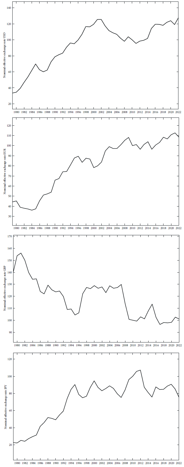
Source: IMF, External Sector Statistics, and International Financial Statistics.
Figure 1 Cycles in the nominal effective exchange rates of major currencies
In this sense, it is significant that Biasco focuses on the major world currencies, those supposedly backed and underpinned by the ‘deeper’ and most modern financial markets. Indeed, after the Global Financial Crisis of 2007-8, the IMF itself started considering capital account liberalization with more prudence and balance -in theory, if not in practice (Gallagher and Ocampo, 2013). But usually these considerations, as those by the bulk of the literature, are typically focused on low- and middle-income countries (see e.g.Botta, 2021). For higher income countries, it is often assumed that financial markets are more integrated, and that monetary policy can be more independent despite freedom of movement of capital, thanks to their larger economies and larger and deeper financial markets (this assumption underlies several analyses of currency hierarchy too).
To our knowledge, the closest mainstream analysis to that presented here that deals with major world currencies is the one developing the notion of a “Global Dollar Cycle” (Obstfeld and Zhou, 2022). It too, however, is framed within the same analysis of the GFC and thus has the same problem of being based on a notion of ‘cycle’ as driven by a sequence of exogenous shocks. Especially but not exclusively among heterodox authors, the other reflections on the role of capital movements in shaping upper-income countries’ currencies have mostly taken on a hypothetical nature, discussing the possible repercussions of a breakup of the euro and/or the exit of some European member state from the currency union, with little empirical analysis of the actual policy space for the central banks of the larger countries.
2.2. The exchange rate level
If the exchange rate is driven by financial movements and there is no equilibrium value for it (or it is not reached in practice), a relevant question is what happens to the real economy as the level of the exchange rate changes. On this point, post-Keynesians are more divided (Blecker, 2023). On the one hand, several authors (for example the Sraffians) are generally suspicious of giving too much prominence to equilibrium adjustments based on the price mechanism rather than changes in quantities. For example, Thirlwall’s Law can be generalized to include appreciation/depreciation as a cause of price competitiveness and thus changes in the import and export elasticities of demand (Thirlwall, 2011); but ever since its original formulation, Thirlwall has rather opted to work without too much emphasis on exchange rate movements, stressing instead the role of changes in national and world GDP and, implicitly, firms’ non-price competitiveness. On the other hand, other authors -again, often with a focus on low- or middle-income countries, such as for example Latin American Structuralism- claim that prolonged periods of a ‘misaligned’ exchange rate can lead to problems in the terms of trade and changes in competitiveness. This is the case for example of the New Developmentalist approach (Palley, 2021; Oreiro and de Paula, 2022; both in this journal). With a focus on developing economies, structuralists argue that depreciation can foster industrial growth by boosting exports, but both mainstream and other post-Keynesian economists contend that long-term growth effects are minimal. For example, among the former Krugman and Taylor (1978) caution that depreciation often raises inflation and constrains growth in poorer countries, and more recently among the latter Ribeiro et al. (2020) found only limited positive effects. According to Blecker (2023), while moderate depreciation can support exports, its impact on broader economic growth remains unclear.
An explicit link between depreciation/appreciation and growth due to the impact of capital movements on the former is found in the notion of a “Financial Dutch Disease” (Botta, 2017, 2021). If large and persistent capital inflows (due to whatever reason) create a strong currency appreciation, Botta et al. (2023) claim that they can initially support an industrial expansion, but they then create strong challenges for all other sectors due to the lack of price competitiveness. This situation mirrors the traditional Dutch Disease, where a single export sector (typically natural resources: Isabella, 2024) appreciates the currency and suppresses other sectors. Rodrik (2016) terms the resulting stagnation or even crisis as “premature deindustrialization”. In this case too, limited research has addressed these dynamics in wealthier economies, although Rapetti et al. (2012) and Berg et al. (2012) provide evidence that prolonged appreciation can limit growth by reducing export competitiveness.
With a focus on emerging economies, the formalization of a model most closely resembling in its final solution the closed form solution of our own (described below) is that by Kohler and Stockhammer (2023). They focus on the impact of the exchange rate on aggregate demand through what they call a “financial channel” whereby depreciations are contractionary due to the weight of foreign-currency debt: “exchange rate appreciation during booms reduces the value of foreign-currency debt, which improves balance sheets and stimulates spending, whereas depreciation induces contractionary deleveraging”. Their key innovation is to combine the financial channel of the exchange rate with an external adjustment channel through which output contractions feed back into exchange rate appreciation, so that endogenous cyclical fluctuations between the exchange rate and output emerge.
Kohler and Stockhammer’s (2023) point is that depreciation against the US dollar tightens borrowing constraints and discourages private spending: This way, a flexible exchange rate regime is not an automatic stabilizer of the economy. This conclusion was certainly shared by Biasco: again, both in the 1987 article and in his other works, but for partly different reasons. For example Biasco (1981) stresses that due to the opposing price and quantity effects of a depreciation, the immediate and automatic impact of a depreciation is a reduction and not an increase in the monetary value of the receipts of exporters. According to the hypothesis of a J-effect (e.g.Lucarelli et al., 2018), over time the quantity effect should gradually prevail until the final impact is positive; but Biasco replies to this approach by noting that in the meantime the monetary and financial, as well as the real conditions of the economy have changed, so that the exchange rate will change again and the hypothetical equilibrium value at which the final effect would have been positive might never be reached. (This is a sort of historical time versus hypothetical time argument that has been often highlighted by the Anglo-Italian School too).
Rather, for Biasco (1987) an indirect link finally producing a positive impact of depreciations on GDP is created by the behavior, in practice, of central banks. Both in the economy with an appreciating currency and in that with a depreciating one, the central banks are bound to react to induced changes in the unemployment and inflation developments (though in the depreciating currency this need for action is stronger and more urgent), and it is rather the change in official interest rates to then impact on the national economies, with later reactions of capital flows and thus of the exchange rates. This is the mechanics that we represent in the model described in section 3.
3. BIASCO ON EXCHANGE RATE CYCLES
Biasco (1987) frames the description of his theory by considering one run of a stylized currency cycle. We will follow his narrative in this section, to showcase the richness of the theory -that is then inevitably lost in a formal model like ours.
Biasco starts from an initial phase of appreciation. The signals guiding this cycle, i.e. driving financial capital into the country and thus producing an appreciation of the currency, can be either monetary/financial or real. The former signals include factors like interest rate differentials, political events, and expected actions by the monetary authorities; while real signals encompass business profitability, competitive strength, export levels, specialization, and inflation rates. Biasco suggests that economic agents with short- to medium-term objectives are primarily influenced by monetary/financial signals, whereas those with a longer-term horizon consider real signals more significant. But most agents tend to focus on short- and medium-term goals for their portfolio, due to uncertainty. Cycle reversals arise when monetary-financial and real signals coincide. This convergence is crucial, as the presence of long-term investors at these moments is essential to initiate a shift in the cycle.
Let us assume that the interest rate is high in this economy. It typically takes time for appreciation to gain substantial momentum because, Biasco argues, economic agents initially struggle to distinguish between temporary and lasting dynamics. As a result, appreciation is approached cautiously, partly due to the adaptive expectations that influence market participants. Only after a sustained period of currency appreciation agents start to substantially increase the allocation of their portfolios to this country, reinforcing the currency’s strength as expectations solidify. Both the monetary and real sectors gradually adjust to this new scenario. The monetary authorities may continue to limit interest rate differentials (i.e. to lower the interest rate) only cautiously, given the positive indications from private operators and the real economy. Meanwhile, the productive sector -at this stage comprising financially robust firms- is still able to adapt, further fueling positive expectations.
As the currency appreciates, inflation declines significantly and persistently, making the real exchange rate increase less than the nominal rate, but this is still insufficient to absorb the growing current account imbalance that is necessarily associated with a net capital inflow. Central banks often accumulate reserves in this stage, which delays trade balance adjustments and enhances the currency’s appeal. Biasco notes that appreciation does not happen all at once because economic agents cannot immediately form expectations of a target medium- to long-term level of the exchange rate based on the evolving positive signals. This uncertainty is heightened as new information emerges regarding the economy’s response to the appreciation.
Over time, a level of appreciation somehow deemed as of “equilibrium” by speculators (fundamentalist traders, in modern parlance) is reached, where the exchange rate stabilizes or rises only modestly. However, this phase is marked by high volatility, which increases market uncertainty and shortens traders’ time horizons, making them shift focus toward monetary rather than real signals. Even long-term investors, due to adaptive expectations, may still remain cautiously optimistic about the future. Even if trade deficits and industrial setbacks were to occur at this point, they may come to be viewed as offset by the low inflation, firms’ high specialization, and the economy’s resilience to a strong currency. Supported by a still rather restrictive monetary policy, the exchange rate remains elevated at this point.
However, deteriorating conditions in the real economy and growing trade deficits eventually compel the central bank to intervene with a significant policy shift. According to Biasco, this intervention is intrinsic to the currency cycle rather than an external shock. As agents with short- and medium-term objectives react to changing financial conditions and monetary policies, they adjust their expectations negatively. They anticipate the direction of the central bank’s intervention, but they cannot predict its scale or timing, leading to shifts in expectations in response to the new expansionary policy. When monetary-financial and real signals converge, even long-term investors reassess their outlook: This is the beginning of the depreciation phase. Biasco highlights two key points here: First, that a convergence of signals is necessary for depreciation to start, and second, that the process is initially gradual but accelerates over time due to strong expectations based on the previous conditions.
At this point, the second half of the cycle proceeds more or less symmetrically to the ascending phase. Rather than delving into the details, it is interesting to ask if one run after the other the cycle always restarts in the same way -or in other words, if there is not a longer-term trend too. Indeed, especially in the article’s concluding section, Biasco explores the impact of the currency cycle on a country’s productive structure, which he considers as interdependent with the currency cycle. Echoing some structuralist themes, according to Biasco during the ascending phase of the exchange rate, the least competitive firms are expelled from the market, and the subsequent recovery during the depreciation does not lead to a re-entry in the market by the very same firms. Therefore, each new run of the cycle starts from a higher average productivity of the economy. This aspect, however, would necessitate its own separate treatment (for more information we refer to Palma, 2023). Consideration for cyclical growth as implied by this last observation would further increase the (already high) number of variables to be considered and we rather leave this aspect for a future work.
3.1. Formalization of the model
We attempt here a formalization of the main elements of the aforedescribed theory, focusing on the following original aspects that emerged from the previous discussion:
endogeneity of instability;
dominance of finance;
bidirectionality of exchange rate and GDP dynamics;
applicability to high-income (very financialized) economies;
discretionary but substantially endogenous monetary policy.
From a methodological point of view, our overarching choice is to investigate the cyclical dynamics that could emerge from the interdependence between GDP, which is a negative function of the exchange rate level (or of its appreciation), and the exchange rate, which is a positive function of (expectations of) GDP growth. To isolate this possible origin of cycles, we deliberately model all functional relations in a simple linear form -even if this might be considered less than realistic, but non-linearities can give rise to further cyclical oscillations by their own (and even chaotic dynamics). Further, we represent the formation of expectations in a simplified and perhaps un-Keynesian way, because it is well known that the interaction between fundamentalist and momentum traders too can by itself give rise to cycles (Gusella and Stockhammer, 2021). In the real world, these two possible origins of cyclical dynamics could reinforce the mechanism investigated here; but our aim is to understand if Biasco’s story per se is a sufficient cause of the emergence of currency cycles such as those displayed in Figure 1.
We consider two countries, A and B, each with its own currency so that one can define the bilateral exchange rate. They could obviously be interpreted as a country (no need for letters in this case) and the rest of the world (RW), in which case we would be referring to the country’s effective exchange rate. In this case, all variables for the rest of the world should be interpreted as a weighted average of the relevant variables for the single economic and financial partners of the country.
Starting from monetary policy, we assume that both central banks, of the country and of the rest of the world, use a Taylor rule to determine official interest rates (i). So the latter depend on the inflation rate (
Assuming for simplicity that the parameters of the reaction functions (σ1 and σ2) are the same for the two central banks, and ignoring the whole structure of interest rates,5 we will refer to the interest rate differential (or spread) between the country and the rest of the world with reference to the central bank determined official rates. The spread is thus easily derived as a function of the difference in the inflation rates and the unemployment rates between the two areas:
Invoking Okun’s Law, we assume that there is a stable relation between the unemployment rate and GDP growth (
Where U is an exogenous component representing any other possible source of differences in the unemployment rate. Here we assume again the same elasticities (λ) in the two countries -as we will do throughout, without further mentioning it (we will not instead assume that the difference in the exogenous variables necessarily disappears, in order to clarify that this is a ceteris paribus analysis, but for simplicity in the determination of differences we use the same symbols as the exogenous variables themselves).
Inflation can be demand-pull -as captured by GDP growth- or cost-push. The former case is the familiar conflict inflation, while in the latter case, the main cause of price changes is ‘imported inflation’ as implied by a depreciation of the exchange rate (e, using the convention that a growing exchange rate represents an appreciation of the country’s currency). The difference in the inflation rates of the two countries is thus:
Where P is an exogenous (differential) component.
Substituting [2] and [3] into [1], and after some manipulation6:
Where P and U now denote the impact of any possible difference respectively in the exogenous components of inflation and unemployment for the two countries7.
The second building bloc of the model are international financial flows. These are driven by investors’ expectations, and operators with different time horizons focus on different variables. The stock of short-term (portfolio) net international positions (IIP ST ) is determined by momentum traders, who focus on the expected relative yield in the country with respect to the rest of the world. The stock of long-term net international positions (IIP LT ) is determined by fundamental traders, who have rational expectations and consider a wider set of variables -summarized here by GDP growth and monetary policy- in order to form expectations on future yields. Evidently, the country’ net international investment position (IIP) is the sum of the short-term and long-term positions.
According to Biasco, momentum traders use technical analysis, which we schematically represent with the assumption of adaptive expectations, denoted in [6] by the superscript e; while for predictions obtained with rational expectations, we use the operator E[.] in [7]. A typical hypothesis on adaptive expectations is to assume that operators consider the immediately previous value of the variable as their prediction for the next one; a reasonable hypothesis on rational expectations in our model is for investors to consider as equilibrium (target) value of a variable its average value over the cycle. With ϑ the fraction of net financial capital mobilized by momentum traders:
However, it is well known that such setup can itself produce endogenous oscillations (Gusella and Stockhammer, 2021); to prevent this, and for simplicity, we assume that both classes of investors continuously update their expectations so that both i e = i and E(i) = i, and the same holds for the expectations about all other variables. In our simplified model, the only difference between the two classes of speculators is the set of variables on which they focus, due to their different time horizons. These assumptions on expectations -in so far as they imply that speculators are always correct -could appear to be anti-Keynesian, but they represent a conservative approach on our side: We are not concerned with the question of whether speculators incur into systematic mistakes and indeed, in order for cyclical dynamics to emerge, we do not need to assume that they do.
Nonetheless, to allow for the theoretical possibility of Keynesian or Minskyan phenomena we add an exogenous component in both cases (respectively denoted by AA ST and AA LT ) to represent changes or shifts in expectations or the state of confidence independent from interest rates or growth rates. But our model is not stochastic, and crucially, it is not based on the interaction between the two classes of investors to produce cyclical dynamics. In the end, if in the real world endogenous financial dynamics produce additional perturbations or even regular cycles, this would only reinforce the meaning of the analysis conducted here -that is to say, that the exchange rate does not converge to a stable equilibrium level and that it exhibits cyclical oscillations.
Plugging [6] and [7] into [5] obtains the economy’s net international investment position:
From which, plugging in the (correct) expectations:
and substituting the interest rate spread from [4] and again economizing on the symbols denoting exogenous variables8:
Finally, we assume that changes in the exchange rate are driven by gross financial flows, which however maintain a certain proportionality (α) with the net values. Denoting absolute changes by a dotted variable:
which suggests that a country growing more than the rest of the world will experience an appreciation due to net inflows of financial capital.
Concerning the other main variable of interest, we assume that income growth, or rather, absolute changes in the growth rate differential between the two economies, are positively affected by the stock of net long-term financial inflows (which, to some extent, might include FDI):
IIP LT can be obtained with the same procedure used for the whole IIP in [8], that is, by starting from [7], assuming correct expectations and substituting for the interest rate spread in [4] (we omit the passages for space reasons), resulting in:
Notice that this time the relation between the exchange rate and the change in the income growth differential, β3 = -ρ2(1 - ϑ)φ4, is univocally negative. This result suggests that the central bank of a country whose currency depreciates will at some point engage in a restrictive monetary policy, which will attract back long-term capital, which is beneficial for the growth differential (if not for growth tout court)9. This result too might at first sight appear as unusual from a Keynesian perspective, but indeed, an increasing number of post-Keynesians are moving in the direction of ruling out a traditional direct GDP impact of monetary policy, arguing instead that the main impact of interest rate changes is on other variables (e.g. on income distribution, according to Seccareccia and Lavoie, 2024). Evidently, the same result as [10], i.e., a negative impact of the exchange rate on the income growth differential, could be obtained by simply assuming that appreciation has a negative impact on net exports, so a more traditional approach (or a Structuralist one) would produce the same result as that presented here, and a crucial question for future research is understanding the channels on which our empirical estimates of β2 (described in the next section) depend.
Jointly, the system of linear differential equations [4] and [10] expresses the gist of the model:
A necessary condition for such system to result in cyclical oscillations is that the terms in the Jacobian matrix’s (J) antidiagonal exhibit opposite signs. A sufficient condition is complex conjugate eigenvalues in the Jacobian, with the signs of the Jacobian main diagonal’s elements differentiating various cycle types. Depending on the value of tr (J), the cycle could converge inward, producing what Gandolfo (1971) terms a stable spiral; it could produce a non-symmetric ellipse: A conservative, closed loop; or an unstable spiral: A divergent, outward-moving cycle. In our model,
As easily seen from equation [8], α1 is positive: That is to say, GDP growth induces expectations of further growth and of appreciation, which drive inflows of capital into the country and thus contribute to determining the expected appreciation itself. β2 has an expected negative sign: Not necessarily because of a direct negative impact of exchange rate appreciation on GDP growth (on which Biasco had several doubts, see section 2) but due to the central banks’ implementation of automatic decision rules that sooner or later compel them to react to imported inflation (arising from a depreciation) with a restrictive monetary policy.
In contrast, concerning the main diagonal there are fewer explicit economic reasons in our model for expecting a certain degree of hysteresis in GDP growth, which would be captured by β1, or for assuming that a high exchange rate would tend to continue appreciating or would reverse course for reasons different from those discussed up to here -except for the compound effect of a series of indirect feedbacks, summarized here by α2. Accordingly, while the model clearly implies cyclical oscillations, if the assumptions above hold, we refrain from making a definite hypothesis on the diverging or converging of these cycles over time, and we will let the data on the single currencies provide information on this aspect.
4. DATA AND EMPIRICAL METHODS
We focus on four main currencies: The dollar, the euro, the pound, and the yen. Research indicates that China’s central bank has actively managed the currency over an extended period, making it unsuitable for the analysis. Japan has also intervened in its exchange rate by accumulating substantial foreign exchange reserves, but its currency is included in this analysis for two reasons. First, while Japan has engaged in significant market intervention, it has not held its exchange rate at a fixed value, enabling an investigation into its currency’s cyclical nature. Second, its interventions are marked by temporal discontinuity. On the whole, for all formally freely floating currencies one must account for a certain degree of dirty floating in reality. As a significant East Asian economy, second only to China in the region, Japan’s inclusion provides valuable context that we think justifies a flexible approach in the inclusion of currencies to study.
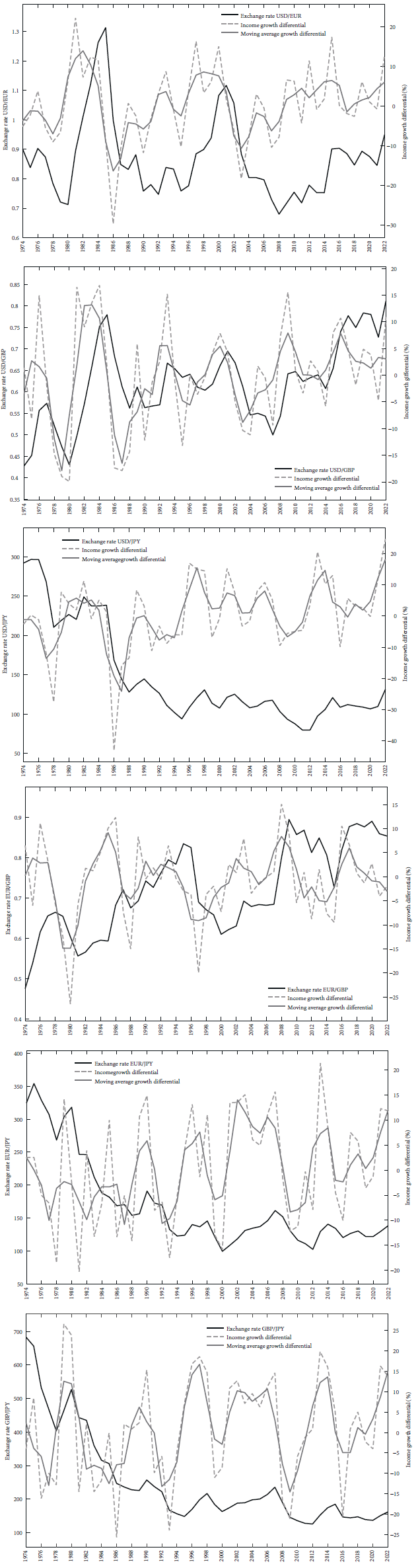
Our analysis spans approximately fifty years of the (formally) flexible exchange rates regime: From the end of the Bretton Woods agreement to the end of 2019, in order to avoid the possible distortions due to the COVID-19 shock from year 2020. Data availability allowed us to work on the period 1974-2019 for all bilateral exchange rates, and on 1979-2019 for the effective exchange rates. Data on nominal exchange rates and nominal GDP in US dollars was sourced from the IMF “External Sector Statistics” and “International Financial Statistics” and the World Bank “Open Data” databases and was considered on an annual basis. Initially, quarterly data was used to enhance robustness thanks to a larger number of observations, but mutual influences between the key variables were observed only with a lag of three-four quarters, indicating a time lag of about one year for the effects described here to materialize. Therefore, for ease of interpretation, yearly data was preferred. For the euro, data before the common currency’s creation in 1999 has been created synthetically, by taking the weighted average of the exchange rate of the single old currencies’ exchange rates and using the respective GDPs as weights.
In addition to examining the six bilateral exchange rates between these major currencies, shown in Figure 2, we also look at the four nominal effective exchange rates, shown in Figure 1 above. While currency-specific trends are evident, these observations indicate that currency markets may indeed exhibit cyclical behavior, as do growth rate differentials (also shown in Figure 2).
For our aims, using the simplest estimation model possible is the most conservative and convenient option, since we are only interested in checking whether the conditions for cyclicality are met, and specifically we are not interested in point estimates or predictions of the relevant variables. Therefore, we employed the following procedure. For all series, we first conducted standard stationarity tests. To ensure consistent VAR analysis, the two variables should not be cointegrated: In case of cointegration between the series, a VECM (Vector Error Correction Model) should be used instead, but this has never been necessary in our case, because the two series are never integrated of the same order.
Next, we tested for structural breaks and for the existence of time trends in the series. In the next section, we show results on detrended series for the subperiods demarked by the estimated structural breaks. Results do not qualitatively change when considering the whole period (1972-2019) for all series, and/or the raw (not detrended) data10.
For each exchange rate, we selected the VAR model that best fits the time series according to the Bayesian Information Criterion (BIC). When the best time lag was one, the estimated coefficients correspond to the Jacobian matrix. However, if the model with the lowest BIC had more than one lag, a special property of cyclic models was used. Stockhammer et al. (2019) show that in this case the necessary and sufficient conditions for cyclicality in the system can be checked by estimating a VAR model and computing the estimated eigenvalues from the coefficients of the first lag matrix only. Cycle length can then be calculated as follows:
Where R is the modulus of the eigenvalue, and h is its real part.
However, for all estimates a further adjustment is needed. Considering for simplicity a simple 1-lag VAR on the two series, it has the following form (denoting the two countries by A and B):
Whereas our interest is in
5. MAIN RESULTS
The analysis of both bilateral and nominal effective exchange rates (NEERS) reveals that these rates do follow cyclical patterns consistent with Salvatore Biasco’s theoretical model. Each exchange rate considered exhibits such cyclical properties, though with variations in stability and the presence of structural breaks over time.
Specifically, Augmented Dickey-Fuller (ADF) tests, reported in Table A1, confirmed the stationarity of all the series of income growth differentials considered, and of a majority of exchange rates (series see statistical annex). Notably, the US dollar/euro bilateral exchange rate and the dollar/sterling rate are found to be not stationary.
Nine out of ten exchange rate series considered exhibit structural breaks, as shown in Table A2. For the dollar/euro bilateral exchange rate we do not find significant structural breaks, allowing for a VAR(1) model to assess cyclical dynamics. For the dollar/sterling rate, structural break tests identify two breaks around 1982 and 2015, prompting a focus on the 1983-2014 period. For the dollar/yen exchange rate, despite the caveat expressed above a cyclical pattern becomes prominent post-1988; due to a structural break around 1985, we consider the 1986-2019 period suitable for VAR analysis. The euro/sterling rate shows an important structural break around 2007; similarly, the euro/yen rate transitions to a cyclical behavior after 1984, with a structural break around 1983. Finally, the sterling/yen rate reflects a two-phase dynamic, with a structural break in 1984 followed by cyclical behavior, so the VAR analysis was conducted for the period 1985-2019. Stationarity tests on the subperiods are shown in Table A3. As shown in Table 1, the VAR results confirm the cyclicity of these exchange rates, with estimated eigenvalues supporting this conclusion. In most cases, there is also evidence of a more or less mildly implosive nature of the cycle.
Table 1 Estimated Jacobian matrices
| e t − 1 | (yˆ A − yˆ B ) t-1 | ||
| USD/EUR | Δe t | -0.287 (0.090)** | 0.343 (0.115)** |
| Δ(yˆ A − yˆ B ) t | -0.355 (0.109)** | -0.629 (0.139)*** | |
| USD/GBP | Δe t | -0.484 (0.110)*** | 0.285 (0.077)*** |
| Δ(yˆ A − yˆ B ) t | -0.941 (0.216)*** | -0.424 (0.139)*** | |
| USD/JPY | Δe t | -0.341 (0.109)** | 34.73 (12.59)** |
| Δ(yˆ A − yˆ B ) t | -0.003 (0.001)** | -0.681 (0.111)*** | |
| EUR/GBP | Δe t | -0.225 (0.091)* | 0.227 (0.076)** |
| Δ(yˆ A − yˆ B ) t | -0.547 (0.190)** | -0.750 (0.159)*** | |
| EUR/JPY | Δe t | -0.402 (0.112)*** | 44.79 (19.88)* |
| Δ(yˆ A − yˆ B ) t | -0.0027 (0.0008)** | -0.716 (0.149)*** | |
| GBP/JPY | Δe t | -0.391 (0.106)*** | 73.00 (26.59)** |
| Δ(yˆ A − yˆ B ) t | -0.0022 (0.0005)*** | -0.587 (0.138)*** | |
| Eff. USD | Δe t | -0.220 (0.088)* | 0.546 (0.184)** |
| Δ(yˆ A − yˆ B ) t | -0.104 (0.094) | -0.565 (0.196)* | |
| Eff. EUR | Δe t | -0.480 (0.150)* | 0.232 (0.158)° |
| Δ(yˆ A − yˆ B ) t | -0.494 (0.167)** | -0.757 (0.176)*** | |
| Eff. GBP | Δe t | -0.143 (0.102)° | 0.388 (0.155)** |
| Δ(yˆ A − yˆ B ) t | -0.248 (0.101)* | -0.657 (0.154)*** | |
| Eff. JPY | Δe t | -0.423 (0.129)*** | 0.319 (0.153)* |
| Δ(yˆ A − yˆ B ) t | -0.447 (0.125)*** | -0.646 (0.149)*** |
Notes: ° significant at p < 0.1, * p < 0.05, ** p < 0.01, and *** p < 0.001. The t-tests for statistical significance are one-sided in order to check whether the coefficients have the expected sign.
Beyond the single bilateral rates, the nominal effective exchange rate (NEER) of the US dollar acts as a benchmark in the global market, with an appreciation indicating an increase in the NEER and depreciation signifying a decline. The Dollar NEER analysis reveals a cyclical pattern similar to bilateral exchange rates, with a long-term trend toward equilibrium. Although the strong upward trajectory initially masks these cycles, detrending the series reveals an implosive cyclical dynamic. The ADF test confirms stationarity in the income growth differential but not in the exchange rate, ruling out cointegration. A structural break around 1993 divides the series into two periods, enabling VAR analysis of the detrended 1993-2019 series, which confirms cyclicity with negative diagonal coefficients in the Jacobian matrix, indicating implosivity.
The Euro NEER, analyzed from a synthetic series for the period before 1999, shows a similar cyclical behavior. The income growth differential for the Eurozone versus global growth generally lags behind global rates, contrasting with U.S. trends. Structural break analysis indicates a break around 1992, allowing the analysis of the 1992-2019 subseries. The VAR model confirms cyclicity, with a Jacobian matrix showing negative diagonal coefficients, implying a move toward equilibrium. The Pound Sterling NEER, unlike other NEERS, reflects a steady depreciation trend over time, although cyclical dynamics are still evident. The income growth differential for the U.K. shows a decline, consistent with a lower growth rate compared to the global average. A structural break around 2008 allows for var analysis on the detrended series, which confirms cyclicity and implosivity.
Lastly, the Yen NEER provides a basis for comparing East-West monetary trends. This rate follows the cyclical patterns observed in the Euro and U.S. dollar, with growth in the late 20th century followed by stabilization. Since 1993, Japan's income growth differential has mostly been negative, reflecting higher global development rates. The VAR analysis for the post-1992 period confirms cyclicity and implosivity, with the Jacobian matrix meeting the criteria for cyclic behavior.
6. CONCLUSIONS
As noted by Biasco (1987), a satisfactory post-Keynesian model of the exchange rate should feature at least: Endogeneity of instability (including expectations, monetary policy, etc.), dominance of finance, and should be relevant for core currencies too. In this work, we sought to check whether theoretically a bidirectionality in the causation between the exchange rate and GDP growth can be postulated starting from fairly post-Keynesian assumptions (and even some anti-Keynesian ones, adopted in order to take a conservative stand), and whether empirically there is evidence of this bidirectionality giving rise to cyclical patterns.
Our analysis reveals that all major bilateral exchange rates and the NEERS of major currencies exhibit cyclicality, often with trends suggesting a gradual stabilization especially among developed economies. In all cases, we find stationarity for income growth differentials, supporting the consistency of cyclical patterns across growth rates. Structural breaks highlight temporal regime shifts in several series, suggesting intervals of significant economic changes. The var analyses also suggest implosive cyclicality in several cases, indicating that both exchange rates and income growth differentials could be moving toward a long-term equilibrium, albeit extremely slowly (that is, over more than forty years, and not even reached yet). Overall, these findings broadly align with Biasco’s theoretical model, which proposes that exchange rates reflect cyclical economic dynamics influenced by both financial flows and monetary policy decisions.
A final clarification could be what is distinctly post-Keynesian in this analysis. We developed the model in a way that cyclical growth not only does not depend on exogenous shocks, but it even does not emerge from non-linearities (à la late Goodwin) or from the interaction between momentum and fundamentalist traders. It rather arises from the endogenous dynamics of international financial flows and the typical reaction of monetary policy. Those other factors, if present, would further amplify oscillations, as would any Minskyan boom-bust dynamics arising from sudden (possibly exogenous) changes in expectations or the state of confidence. Therefore, according to our analysis the normal functioning of a freely floating exchange rate regime in a highly financialized economy is all is necessary for the economy to exhibit instability, in the form of cyclical dynamics. Further research is needed, to understand if the observed correlations between exchange rates and growth differentials actually arise due to the specific mechanisms postulated here, and not some others assumed in the literature, in particular concerning the negative impact of appreciations and the GDP impact of interest rate changes.

