


 nueva página del texto (beta)
 Inglés (pdf)
 Artículo en XML
 Referencias del artículo
 Enviar artículo por email
 Citado por SciELO
  Similares en
SciELO
Similares en
SciELO 
 Permalink
1. INTRODUCTION
In the last three decades, Latin America has experienced a significant decline in its infrastructure assets, both in terms of quality and quantity, relative to other developed and developing regions. Despite the diversity among Latin American countries, this phenomenon has affected nearly all infrastructure sectors in the region. For instance, Calderón and Servén (2002) estimated an increase in the infrastructure gap in Latin America compared to the Asian Tigers, ranging from 40% to 50% in road infrastructure, 50% to 60% in telecommunications, and 90% to 100% in terms of electrical generation capacity.
The deterioration of infrastructure leads to its overuse and the emergence of increasing bottlenecks in service provision. This situation adversely affects productivity, escalates costs, and diminishes profit expectations, thereby hindering private investment. Through these various channels, the ultimate consequence is reduced economic growth. Additionally, Calderón and Servén (2002) demonstrated that the disparity in Gross Domestic Product (GDP) per worker (adjusted by Purchasing Power Parity, PPP) between East Asia and Latin America expanded by approximately 90% between 1980 and 1997. Pressures for fiscal consolidation in Latin American countries typically resulted in reduced public spending on infrastructure, which was not offset by an increase in private sector participation (Carranza and Melguizo, 2014), ultimately leading to an insufficient provision of infrastructure services with adverse effects on productivity and growth1.
The aim of this article is to present an empirical analysis of the infrastructure sector’s contribution to GDP growth and productivity within specific groups of countries. More specifically, we compiled a dataset of indicators measuring the extent of physical infrastructure, encompassing 18 countries in Latin America and the commonly referred to Asian Tigers, for the period 1980-2017. The study primarily focuses on estimating the impact of infrastructure stock, derived through Principal Component Analysis (PCA), on both GDP and the productivity of private factors. Essentially, we seek to assess the long-term influence of infrastructure capital on GDP and total factor productivity (TFP). Several critical questions will be explored: Is there a long-term relationship between this infrastructure stock and GDP within this set of countries? If such a relationship exists, which group of countries demonstrates the highest GDP growth concerning infrastructure? Does infrastructure stock significantly affect the productivity of private production factors? If so, what is the magnitude of this impact for these two groups of economies? Finally, the causality between the infrastructure stock and GDP is investigated; and also between infrastructure stock and productivity. Changes in the infrastructure stock precede changes in GDP (or productivity) or the other way around? Was the recession that occurred at different times in these economies due to the fall in investments or did the recession itself generate a fall in investments? What is the direction of causality? This is an important issue since, to analyze income elasticity, it is assumed that the dependent variable is GDP and the independent variable is the infrastructure stock.
We have some contributions to the literature, in our view. First, we add one more element in the discussion of the different paths of Latin American countries and the Asian Tigers in terms of catching-up. Second, we update the impact of infrastructure in these regions based on a more recent period (between 1980 and 2017). Third, we use other methods to build the aggregate indexes of infrastructure and to estimate its effects on GDP and productivity. For instance, we use some estimators that consider heterogeneous coefficients and cross-section dependence between the panel units. To our knowledge, this methodology has not been used by other studies on this present topic. The results support the view in other studies about the importance of infrastructure on GDP and productivity, as we will see in the following sections. And, in fact, it could be one of the reasons of the different GDP trajectories of Latin American countries and the Asian Tigers.
This article is organized as follows. Section 2 provides a concise review of the relationship between infrastructure and economic growth, along with empirical findings from prior studies focusing on the primary topic of this work. In section 3, we present the methodology of econometric analysis and the database used. The empirical results are in section 4. In section 5, we have the final considerations of the article.
2. PHYSICAL INFRASTRUCTURE, ECONOMIC GROWTH, AND THEIR IMPACTS: A BRIEF REVIEW
The presence of adequate infrastructure stock is crucial for fostering sustainable growth. Notably, scholars such as Nurkse (1953), Scitovsky (1954), Rosenstein-Rodan (1943), and Hirschman (1958) have highlighted the relationship between infrastructure, externalities, and economic growth. According to Lewis (1979), growth necessitates both infrastructure and trained human resources, even in nations primarily exporting primary products. Additionally, certain studies indicate that disparities in income levels and growth rates among countries stem from activities that generate externalities. Hence, nations that effectively provide the right incentives and foster activities generating externalities tend to experience rapid growth and achieve a higher standard of living compared to other countries.
Physical infrastructure serves as a significant example of externality, as it facilitates industries’ access to increasing returns. The construction of infrastructure often leads to substantial production growth, as many industries expand upon gaining access to it, benefiting from cost reductions and productivity enhancements2. An intriguing example is the American experience with railroads. Murphy, Shleifer and Vishny (1989) put forth a model wherein infrastructure is linked to a significant surge in industrialization. Many companies leveraging it for production and hiring create substantial external benefits for each other, as previously described. Furthermore, drawing on the notion of complementarity or congestion in infrastructure allocation, given its scarcity, one can argue that the private capital stock becomes more productive when ample infrastructure services are available. Conversely, inadequate allocation of infrastructure capital may lead to suboptimal relations between infrastructure and private capital in the country3.
In a seminal article, Aschauer (1989a) estimated that an increase of 1% in public capital in infrastructure would imply an increase of between 0.36 and 0.39% in the product for the American economy. Munnell (1990) finds similar estimates with regional American data. With another series of infrastructure (containing streets, highways, gas and electricity services, water and sewage systems and mass public transport), Aschauer (1989b) found an income elasticity of 0.24. Uchimura and Gao (1993) found GDP elasticities with respect to infrastructure capital of 0.19 for Korea and 0.24 for Taiwan. Additionally, Shah (1992) found a value of 0.05 for Mexico.
For the Brazilian case, the work of Ferreira and Malliagros (1998) is one of the precursors. The authors point out that for a 1% increase in infrastructure capital productivity increases vary from 0.482% to 0.49%. Thus, they concluded that the fall in factors’ productivity observed since the 1980s in Brazil is explained by the reduction in infrastructure investments which occurred in the period. Mussolini and Teles (2010) try to capture a possible “congestion” effect in public services by verifying the relationship between the public capital/private capital (G) ratio and TFP. When confirming that these variables series are co-integrated, a Vector Autorregression (VAR) is made and it is verified that an increase of 1% in G causes, in the Granger sense, a rise between 1.6% to 2.5% in TFP in the long term -depending on the measure used to calculate TFP. The authors also conclude that the elasticity of TFP in relation to public capital would be between 0.32 and 0.5. That is, fiscal adjustments based on the contraction of such investments could compromise the longer-term fiscal framework through the economic growth channel (considering TFP as one of the fundamental variables for the long-term growth of an economy).
Ingram (1994) estimated elasticities for several sectors (installed kilowatt, kilometres of paved roads and installed telephones, etc.) for 100 developing countries. The results indicated that telecommunications, electricity, highways, irrigation, sewage systems, piped water systems and railways (in decreasing order) are the sectors that most influenced GDP.
Regarding causality, for the American economy, Ferreira and Issler (1995) concluded that variations in public infrastructure spending precede variations in total factor productivity, and the inverse relationship is rejected. On the other hand, Easterly and Rebelo (1993) show that there is no evidence of substitutability between public investment in infrastructure and private investment. Belloc and Vertova (2004) pointed out that the complementarity between public investment in infrastructure and private investment involves not only Total Factor Productivity, but also increased demand through a larger market and profit expectations.
Álvarez-Ayuso, Becerril-Torres and Moral-Barrera (2011) estimate the productivity of Mexican states (dividing in terms of technology and efficiency) and build a productivity indicator based on categories of transport (highways, ports and airports), telecommunications and availability of water and electricity. The authors find, using panel data, that the increase in infrastructure positively impacts the growth in private production factors -particularly on the technical component. Sahoo, Dash and Nataraj (2010), create an infrastructure index with six items (electricity consumption, oil consumption, telephone lines, density of railways, air transport, paved roads). They find infrastructure elasticities on GDP vary between 0.20 and 0.41.
Furthermore, Calderón and Servén (2012) observe the effects of infrastructure on productivity in Latin American countries in comparison to other groups of countries. These countries had their growth increased by only 0.32 percentage points (pp) between 1986-1990 compared to 1976-1980 due to the development of infrastructure; much lower, for example, to East Asian countries, with an increase of 1.93 pp annually for the same period. The authors still estimate 2 pp more in the annual growth rate that would be increased if the infrastructure gaps were reduced.
Finally, Liddle and Huntington (2018) estimate the income elasticity of energy consumption with a heterogeneous dynamic panel for 37 OECD (Organisation for Economic Cooperation and Development) and 41 non-OECD countries. Most results suggest that the elasticity of GDP is less than the unit -that is, the energy intensity will fall with economic growth. A “large average” (average of many panel averages) suggests a GDP elasticity of around 0.7. Still, most of the evidence suggests that GDP elasticity is similar for OECD and non-OECD countries, and for non-OECD countries across different income brackets.
3. MODEL SPECIFICATION AND DATABASE
The empirical strategy involves estimating equations to obtain the income elasticity of the infrastructure stock and elasticity of the infrastructure stock in relation to the TFP. So, we adopt the following long-term relationship:
Where, for each country i, GDP i,t = Real GDP at constant 2011 national prices, built upon private investment flows from Penn World Table version 9.1 database calculated according to purchasing power parity (international prices), which corrects the effects of systematic differences in cost of living between economies. (infrastructure stock) i,t = PCA sectors are: i) length of the train line, length of the paved road in kilometers, taken from Canning (1999), IRF (s.f.) and World Bank (2019); ii) fixed-line and Mobile cellular subscriptions, from Canning (1999) and World Bank (2019); iii) generation of Gigawatt electrical capacity (GW), obtained in Canning (1999) and World Bank (2019).
The control variables are: GAP
i,t
= Output Gap (a proxy for the state of economic cycles), estimated through the Hodrick-Prescott filter (HP); the Real GDP at constant national prices (World Bank, 2019); GDP
e
= the expected GDP. In order to estimate the expected GDP
e
, which is not observed, we use the strategy of Erden and Holcombe (2005), a first order autoregressive model, AR (1), the real GDP logarithm is estimated.
TFP is usually measured based on Hick’s Neutrality. Under the Solow’s model production function, Y = AF(K, L), a Hicks-neutral change is one which only changes A. Therefore, to analyze the effect of the infrastructure stock on TFP, one should measure TFP excluding the infrastructure in capital stock K.
Following Canning (1999) and Calderón and Servén (2002), we adopt a Cobb-Douglas specification of the infrastructure-augmented production function:
Where y is the GDP, k is the physical capital stock without infrastructure, l denotes labor, h is human capital, and z is a measure of infrastructure capital. All variables are expressed in logs and constant returns to scale are assumed. Equation [3] assumes that infrastructure services are a fixed proportion of the infrastructure capital stock.
In principle, infrastructure capital appears twice in equation [3] -as part of k, and separately as z. Hence, the parameter γ captures to what extent the productivity of infrastructure exceeds (if > 0) or falls short (γ < 0) of the productivity of non-infrastructure capital (Calderón and Servén 2002).
The contribution of infrastructure capital to output can be found by noting that the measured capital stock is a weighted sum of infrastructure and other physical assets, with weights given by their respective relative prices. Thus, letting
Where uppercase letters denote the anti-logs of lowercase variables; and p z is the relative price of infrastructure capital in terms of non-infrastructure capital. Assuming that the latter is approximately equal to the price of overall capital, under the presumption that infrastructure assets are typically a small fraction of the total capital stock.
Combining [3] and [4], the elasticity of output with respect to infrastructure can be expressed as:
Where:
That is, the share of infrastructure in the overall physical capital stock. These expressions involve log-linear approximations around an arbitrary point (e.g., the sample mean). In practice, since infrastructure stocks typically account for relatively small portions of the overall capital stock, the difference between η z and the ‘naice’ estimate γ should be fairly modest (Canning and Bennathan, 2000; Calderón and Servén, 2002).
For our purposes, since we are primarily interested in the performance of Latin American countries and the so-called Asian Tigers, we compute the capital stock shares using the cost data available for countries in this region and the average ratios of the relevant stocks over 1980-2017, using cost of infrastructure assets collected by Canning and Bennathan (2000). Given the uncertainty of the calculations and as our results were not far from those found by Calderón and Servén (2002), we chose to use the results found by the authors, however, the results have to be taken carefully, and not in a definite way. According to the authors, telecommunications infrastructure accounts for just over 1 percent of the overall capital stock, while power and roads and railroads represent 14 and 16 percent, respectively, for instance4.
In possession of these values, in order to construct the TFP series, we subtract the total capital series from the infrastructure capital, according to their respective shares in the private capital stock.
The total factor productivity (TFP i,t ) which is defined by:
Where Y t is the product -Real GDP at constant national prices obtained (World Bank, 2019); K t is private capital obtained in IMF (2017) and L t is the work- constructed using the occupied population as a proxy5 (World Bank, 2019).
The coefficients α and β indicate the participation of capital and labor in the product, respectively. We will work with α and β of, respectively, 0.4 and 0.6 (following international evidence, as Cooley and Prescott, 1995) and assume constant returns to scale6.
The econometric exercise is carried out for the period 1980-2017 for 18 countries and for two subgroups of countries, from Latin America and Asian Tigers. The countries are: Argentina, Brazil, Chile, Colombia, Ecuador, Guatemala, Mexico, Peru, Uruguay, China, Singapore, South Korea, Philippines, Hong Kong, Indonesia, Japan, Malaysia and Thailand.
3.1. Methodology
Equations [1] and [2] can be estimated by applying three estimators: Mean-group (MG) by Pesaran and Smith (1995), pooled mean group (PMG) by Pesaran, Shin and Smith (1999) and dynamic common correlated effect estimator by Chudik et al. (2016).
Pesaran and Smith (1995) present the estimation of the Autoregressive Distributed-Lags Model (ARDL) as a new cointegration test. The ARDL approach allows for consistent and efficient estimates of the parameters in a long-term relationship between the integrated and stationary variables and to conduct inference on these parameters using standard tests (Pesaran, Shin and Smith, 1999).
According Hsiao, Pesaran and Tahmiscioglu (1999) is an example of heterogeneous dynamic panels showing that the MG estimator is asymptotically normal for large N and T, since
For Ditzen (2019), long run relationships describe the steady state solution and how a change in the steady state affect the long run relationship between variables. Our long run estimates intend to estimate coefficients which capture this kind of relationship. The purpose of common correlated effects estimators is to add cross-sectional averages that approximate the cross-sectional dependence8.
Our estimates were developed using the XTPMG routine proposed by Blackburne and Frank (2007) and the version XTDCCE2 by Ditzen (2018; 2019) 9.
To examine the direction of causality between infrastructure and GDP, and infrastructure and TFP, we used the Causality Test proposed by Holtz-Eakin, Newey and Rosen (1988). The system is known in the literature as Panel Vector Autorregression (PVAR):
Where, I represents countries and t represents the time period, while GDP it and TPF it are in logarithms. infrastructure stock i,t = PCA and is normalized and in logarithm also. α1 and α2 are the intercepts common to the countries. τ1i and τ2i are fixed effects that capture the individual heterogeneity of states and are constant over time, and k denotes the lag that varies from 1 to k. The advantage of this methodology is that it is a reference model for a dynamic panel causality test. In addition to the fact that the empirical analysis of the impact of infrastructure on growth and productivity is already relevant in itself. A second contribution to the literature is the use of estimators that consider heterogeneous coefficients and cross-section dependence between the panel units. To our knowledge, this methodology has not been used by other studies in this regard.
With regard to Granger’s causality hypothesis, this is verified from the Wald test in the Holtz-Eakin, Newey and Rosen (1988). It is a test of restrictions applied to the parameters of the estimated model. In this way, there will be one-way Granger causality from the infrastructure stock to GDP if not all β1i’s are equal to zero in the first equation, but all γ2i’s equal to zero in the second equation. Conversely, there will be one-way Granger causality from GDP to infrastructure stock if all β1i’s are equal to zero in the first equation, but not all γ2i ’s are equal to zero in the second equation. There can be two-way Granger causality between GDP and infrastructure if not all β1i’s and not all γ2i’s are equal to zero. Finally, there may be situations in which there is no Granger causality between infrastructure and GDP, as long as the β1i ’s and all γ2i’s are equal to zero10.
The set of procedures performed is: Cross-section dependency test (CD) by Pesaran (2004); Stationarity tests (Maddala and Wu, 1999; Pesaran, 2007); Cross-section Augmented Dickey-Fuller (CADF) test proposed by Pesaran (2007) is also used; it deals with the case where cross-sectional dependence arises from the presence of a single common factor among the cross-sectional units, cointegration (Pedroni, 1999 and Westerlund and Edgerton, 2008) and long-term estimators and causality tests.
4. EVIDENCE OF THE RELATIONSHIP BETWEEN INFRASTRUCTURE, GDP AND TFP
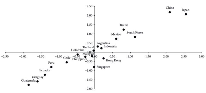
The infrastructure stock aggregate index is composed of the following items: number of fixed and mobile lines subscriptions; electricity generation in GW; and total roads and railways in kilometers11. The indicator has been normalized. It was found that the first principal components generated from this analysis has eigenvalues higher than one (λi > 1) [Kaiser, 1958] and is responsible for 65.57% of the total variance of the five infrastructure stock measures. Therefore, the first main components of the indexes effectively summarize the total sample variance and is presented in the equations below:
Where (infrastructure stock) i,t represent the first principal components of the infrastructure stocks; (Z 1/A) it is the sum of the length of roads and railways in kilometers normalized by the country’s surface area (km per sq. km); (Z 2/L) it is the electricity generation (in GW per 1,000 workers); (Z 3/L) it is the sum of the number of landline telephone subscriptions and mobile phones subscriptions (per 1,000 workers).
Graph 1, below, show the countries’ dispersion according to infrastructure stock. The countries’ dispersion analysis is based on the scores (1980-2017). It is observed that the index can discriminate between infrastructure stocks in less developed countries and those in more developed ones, as it assigns higher values to infrastructure stocks in wealthier nations.
The results of the CD tests by Pesaran (2004) show that infrastructure, GDP and TFP are highly dependent on all eighteen countries -the hypothesis of no correlation is rejected at the usual levels of statistical significance (Annex, Table A1). Descriptive analysis aids in identifying the considerable heterogeneity within the sample data. A mean exceeding the median suggests that values at the upper end of the distribution diverge significantly from the center, relative to values at the lower end. Productivity values exhibit relatively minor differences between the two groups of countries, albeit slightly higher in Latin American countries. Conversely, for other variables, such as infrastructure, values are substantially higher in the Asian Tigers countries. In summary, countries display significant variability in income and infrastructure (see Annex, Table A2).
The results of Maddala and Wu (1999) and Pesaran (2007) stationarity tests, considering 5% of significance, including or not a deterministic trend and with lags ranging from 0 to 2, suggest the non-stationarity of the series (Annex, Table A3 and A4). The result of unit root test in the presence of cross-section dependence, CADF test (Pesaran, 2007), also followed the previous results (Annex, Table A5). The results of the four tests that make up the procedure proposed by Westerlund and Edgerton (2008) suggest the rejection of the null hypothesis of non-cointegration. The results of Pedroni Cointegration test (1999) also indicate a cointegration relationship (Annex, Table A6).
Table 1 presents the results of the estimates using the MG, PMG and XTDCCE2 estimators12, together with the Hausman test to measure the efficiency and consistency between them. The Hausman test validated the null hypothesis of long-term homogeneity restriction of the regressors, indicating PMG as a more efficient estimator than MG. As the homogeneity hypothesis of the slope was accepted empirically, only long-term results are discussed and presented. According to the PMG estimator result, the adjustment speed is -0.167. In the same raw, the CD Statistic results corrected the problem of cross-sectional dependence. According to the estimator results, all the estimated coefficients are statistically significant at least at 5%.
Table 1 Long-term estimates, 1980-2017
| Variables | PMG | MG | XTDCCE2 (PMG) | XTDCCE2 (MG) | ||||
|---|---|---|---|---|---|---|---|---|
| Coefficients | p-value | Coefficients | p-value | Coefficients | p-value | Coefficients | p-value | |
| 18 countries | ||||||||
| GDP | ||||||||
| Long run coefficients | ||||||||
| Infrastructure stocks 1 | 0.446 | 0.000 | 0.932 | 0.034 | 0.561 | 0.000 | 0.958 | 0.019 |
| Adjustment speed/CD statistic | -0.167 | 0.001 | -0.123 | 0.000 | -0.240 | 0.214 | -2.020 | 0.508 |
| Hausman test | 0.440 | 0.508 | 0.180 | 0.672 | ||||
| TFP | ||||||||
| Long run coefficients | ||||||||
| Infrastructure stocks 1 | 0.203 | 0.000 | 0.069 | 0.006 | 0.086 | 0.347 | 0.059 | 0.041 |
| Adjustment speed/CD statistic | -0.113 | 0.000 | -0.236 | 0.000 | -2.890 | 0.003 | -1.000 | 0.146 |
| Hausman test | 4.550 | 0.032 | 9.540 | 0.022 | ||||
Note: The estimates were developed using the XTPMG routine proposed by Blackburne and Frank (2007) and the version by XTDCCE2 (Ditzen, 2018; 2019).
Source: Authors’ elaboration.
The impact of the infrastructure stock taken from the PCA -composed of physical infrastructure measures -on the long-term product has an average coefficient of 0.5035 for PMG and XTDCCE2 (PMG), respectively. This means that an increase of 1% in the infrastructure stock generates an increase of 0.50 pp in GDP in the long run, considering the 18 countries in our sample. The results indicate that investment in infrastructure has a major influence on GDP. The results obtained are similar to the work of Easterly and Rebelo (1993) for cross-section data from developing countries, where they found values for the transport and communication sector of 0.59 and 0.66 respectively13.
The impact of infrastructure stock on long-term TFP showed an average coefficient of 0.064 for PMG and XTDCCE2 (PMG). Thus, a 10% increase in the infrastructure stock produces an increase of 0.64 pp in TFP in the long run.
For comparison, Kim and Loayza (2017) constructed an index combining the main components that would impact TFP, namely, indicators of innovation, education, market efficiency, physical infrastructure and institutional infrastructure for 65 countries in the period from 1985 to 2011 The coefficient found in relation to productivity was 0.020. The authors found values of 0.13 for the subgroup of countries in East Asia and the Pacific and 0.08 for the subgroup of Latin America and the Caribbean. These results are similar to those found for our subgroups for Latin American and the Asian Tigers.
Table 2 shows the results for the Latin American and Asian Tigers subgroups. According to the results, all estimated coefficients are statistically significant at least at 10%. The only exception is the XTDCCE2 (PMG) estimator for the TFP regression.
Table 2 Long-term estimates, 1980-2017
| Variables | PMG | MG | XTDCCE2 (PMG) | XTDCCE2 (MG) | ||||
|---|---|---|---|---|---|---|---|---|
| Coefficients | p-value | Coefficients | p-value | Coefficients | p-value | Coefficients | p-value | |
| Latin American countries | ||||||||
| GDP | ||||||||
| Long run coefficients | ||||||||
| Infrastructure stocks1 | 0.616 | 0.000 | 0.502 | 0.000 | 0.482 | 0.000 | 0.564 | 0.000 |
| Adjustment speed/CD statistic | -0.095 | 0.001 | -0.176 | 0.000 | -1.150 | 0.158 | -1.130 | 0.141 |
| Hausman test | 5.220 | 0.022 | 347.86 | 0.000 | ||||
| TFP | ||||||||
| Long run coefficients | ||||||||
| Infrastructure stocks 1 | 0.070 | 0.008 | 0.053 | 0.179 | 0.072 | 0.101 | 0.052 | 0.383 |
| Adjustment speed/CD statistic | -0.191 | 0.000 | -0.338 | 0.000 | -1.480 | 0.123 | -1.580 | 0.133 |
| Hausman test | 0.370 | 0.540 | 3.230 | 0.357 | ||||
| Asian Tigers | ||||||||
| GDP | ||||||||
| Long run coefficients | ||||||||
| Infrastructure stocks 1 | 0.672 | 0.000 | 1.363 | 0.122 | 0.487 | 0.055 | 0.568 | 0.000 |
| Adjustment speed/CD statistic | -0.077 | 0.003 | -0.069 | 0.000 | -1.600 | 0.123 | -1.580 | 0.113 |
| Hausman test | 0.180 | 0.670 | 0.000 | 1.000 | ||||
| TFP | ||||||||
| Long run coefficients | ||||||||
| Infrastructure stocks 1 | 0.121 | 0.000 | 0.102 | 0.000 | 0.635 | 0.244 | 0.086 | 0.003 |
| Adjustment speed/CD statistic | -0.130 | 0.000 | -0.174 | 0.000 | -1.560 | 0.137 | -1.660 | 0.147 |
| Hausman test | 1.090 | 0.296 | 7.240 | 0.064 | ||||
Note: The estimates were developed using the XTPMG routine proposed by Blackburne and Frank (2007) and the version by XTDCCE2 (Ditzen, 2018; 2019).
Source: Authors’ elaboration.
The impact of physical infrastructure measures on the long-term product for Latin American countries was 0.533 for MG and XTDCCE2 (MG). For the Asian Tigers subgroup, it was 0.5795 for PMG and XTDCCE2 (PMG)14.
In summary, the infrastructure index series cointegrate indicating the existence of a long-term relationship with GDP. The coefficients have the expected sign and the magnitude of the estimated coefficients implies a strong impact of infrastructure on long-term GDP, for the sample and the subsample of countries.
For a simple comparison between the two subgroups of countries, we take the series of: Electricity generation, length of railways and total roads in kilometres, total fixed and mobile phone subscription. We normalized for 1 million people and extracted simple averages for the two subgroups of countries. The average of Asian Tigers is 4.96 times higher in electricity generation, 7.65 times in the length of roads and railways, and 3.72 times in fixed and mobile phone subscriptions. As we note that there are no significant differences in income elasticities between these two groups of countries, we conclude that the greater growth of the Asian Tigers in relation to the Latin American countries in our sample is largely explained by the greater infrastructure stock of the first group.
The impact of infrastructure stocks on long-term TFP for Latin American countries was 0.071 for PMG and XTDCCE2 (PMG). For the Asian Tigers subgroup, it was 0.1035 for PMG and XTDCCE2 (PMG)15.
The results suggest that the impact on productivity is 0.71 and 1.035, respectively, for the Latin American and Asian Tigers subgroups for a 10% increase in the infrastructure stock. This means that a fall in investments in infrastructure will have a negative impact on the factors’ productivity in the long run, as observed, in general, in the last three decades in Latin American countries. Thus, this presents itself as another reason for the lower growth of this region and the fall in productivity of most of these countries.
It is worth noting that our infrastructure index series presented a correlation coefficient with respect to the public capital stock (IMF, 2015) of 79.1% and 73.04% respectively, for the Latin American countries and Asian Tigers, in the period 1980-2016. Thus, our infrastructure stock, in a way, acts as a proxy for public capital stock.
Therefore, enhanced infrastructure, encompassing improved roads, railways, energy, and communication systems, not only amplifies overall output but also augments factor productivity, resulting in cost reductions and instilling greater confidence among business leaders, thereby stimulating investments. Consequently, these results highlight the pivotal role played by infrastructure in driving the growth of private sector productivity. Finally, the causal relationship between the infrastructure stock and GDP is analyzed; and, also, between the infrastructure stock and the TFP (Table 3).
Table 3 Holtz-Eakin causality test - Infrastructure, GDP and TFP
| 18 countries (1980-2017) | |||
|---|---|---|---|
| Infrastructure statistic → GDP | GDP → Infrastructure statistic | ||
| Wald Statistic | 14.446*** | Wald Statistic | 23.809*** |
| Infrastructure statistic → TFP | TFP → Infrastructure statistic | ||
| Wald Statistic | 9.194*** | Wald Statistic | 17.850*** |
| Latin American countries (1980-2017) | |||
| Infrastructure statistic → GDP | GDP → Infrastructure statistic | ||
| Wald Statistic | 3.361* | Wald Statistic | 3.385* |
| infrastructure statistic → TFP | TFP → Infrastructure statistic | ||
| Wald Statistic | 7.240*** | Wald Statistic | 1.898 |
| Asian Tigers (1980-2017) | |||
| Infrastructure statistic → GDP | GDP → Infrastructure statistic | ||
| Wald Statistic | 2.608* | Wald Statistic | 7.091*** |
| Infrastructure statistic → TFP | TFP → Infrastructure statistic | ||
| Wald Statistic | 4.678** | Wald Statistic | 21.757*** |
Notes: *** significant at 1%; ** significant at 5% and * significant at 10%. Chose the number of lags based on Aic/Bic/Hqic and using the Genghurion University Anat Techtchik code. After fitting a panel var model with PVAR, the complementary matrix modules based on the estimated parameters were calculated.
Source: Authors’ elaboration.
We can draw the following conclusions: The infrastructure stock Granger-causes GDP and vice versa, in the three cases -for the whole group of countries, for the subgroup of Latin America and the Asian Tigers. The infrastructure stock causes the productivity of private factors for all countries and for the two subgroups of countries. However, the opposite is not the case only in the subgroup of Latin American countries.
Given that the first principal component generated by the index accounted for 66% of the total variation in infrastructure stock measures, a second infrastructure index was constructed to assess the robustness of the results. This second index incorporates electricity generation in gigawatts (GW) and the number of fixed and mobile telephone subscriptions. The first Principal Component derived from this second index explained 92% of the total variation in infrastructure stock measures, respectively. The results for all countries and subgroups are presented in Table 4.
Table 4 Long-term estimates, 1980-2017
| Variables | PMG | MG | XTDCCE2 (PMG) | XTDCCE2 (MG) | ||||
|---|---|---|---|---|---|---|---|---|
| Coefficients | p-value | Coefficients | p-value | Coefficients | p-value | Coefficients | p-value | |
| 18 countries | ||||||||
| GDP | ||||||||
| Long run coefficients | ||||||||
| Infrastructure stocks 2 | 0.439 | 0.000 | 0.584 | 0.000 | 0.555 | 0.000 | 0.492 | 0.000 |
| Adjustment speed/CD statistic | -0.147 | 0.001 | -0.236 | 0.000 | -0.370 | 0.227 | -2.000 | 0.045 |
| Hausman test | 9.130ª/ | 0.107 | 2.630ª/ | 0.452 | ||||
| TFP | ||||||||
| Long run coefficients | ||||||||
| Infrastructure stocks 2 | 0.089 | 0.000 | 0.068 | 0.006 | 0.061 | 0.049 | 0.063 | 0.052 |
| Adjustment speed/CD statistic | -0.070 | 0.000 | -0.238 | 0.000 | 1.140 | 0.110 | -1.120 | 0.264 |
| Hausman test | 2.45ª/ | 0.117 | 2.53ª/ | 0.469 | ||||
| Latin American countries | ||||||||
| GDP | ||||||||
| Long run coefficients | ||||||||
| Infrastructure stocks 2 | 0.502 | 0.000 | 0.493 | 0.000 | 0.476 | 0.000 | 0.417 | 0.000 |
| Adjustment speed/CD statistic | -0.105 | 0.002 | -0.165 | 0.000 | -0.190 | 0.840 | -0.180 | 0.823 |
| Hausman test | 0.050 | 0.819 | 2.530 | 0.469 | ||||
| TFP | ||||||||
| Long run coefficients | ||||||||
| Infrastructure stocks 2 | 0.083 | 0.000 | 0.094 | 0.314 | 0.092 | 0.121 | 0.055 | 0.405 |
| Adjustment speed/CD statistic | -0.162 | 0.000 | -0.258 | 0.000 | -1.630 | 0.140 | -1.640 | 0.143 |
| Hausman test | 0.020 | 0.899 | 0.000 | 1.000 | ||||
| Asian Tigers | ||||||||
| GDP | ||||||||
| Long run coefficients | ||||||||
| Infrastructure stocks2 | 0.502 | 0.000 | 0.494 | 0.000 | 0.471 | 0.084 | 0.835 | 0.000 |
| Adjustment speed/CD statistic | -0.105 | 0.002 | -0.164 | 0.000 | -0.172 | 0.780 | -0.190 | 0,84 |
| Hausman test | 0.826 | 0.050 | 2.420 | 0.475 | ||||
| TFP | ||||||||
| Long run coefficients | ||||||||
| Infrastructure stocks2 | 0.112 | 0.000 | 0.109 | 0.000 | 0.096 | 0.008 | 0.078 | 0.041 |
| Adjustment speed/CD statistic | -0.131 | 0.000 | -0.180 | 0.000 | -1.570 | 0.133 | -1.640 | 0.143 |
| Hausman test | 0.410 | 0.523 | 0.610 | 0.893 | ||||
Note: a/ Indicates which estimator is more efficient in relation to the Hausman test.
Source: Authors’ elaboration.
The findings (Table 4) demonstrate a remarkable degree of similarity and consistency with those reported in the main models (Tables 1 and 2), albeit with a minor average increase in the estimated elasticities.
5. CONCLUDING REMARKS
Conducting an empirical analysis of infrastructure’s influence on growth and productivity is inherently valuable. Furthermore, comparing Latin American countries with highly successful Asian nations adds an additional layer of compelling interest. Additionally, this article contributes to the existing literature on infrastructure, growth, and productivity by introducing estimators that account for heterogeneous coefficients and cross-section dependence among the panel units. To the best of our knowledge, this methodology has not been utilized in prior studies on this subject.
The results obtained confirm the existence of a strong relationship between infrastructure and gdp in the long term within the sample economies. Furthermore, the long-term estimates of TFP elasticities concerning infrastructure stock are notable. Specifically, the impact of physical infrastructure measures on long-term gdp averaged 0.511 for Latin American countries and 0.533 for the Asian Tigers. Regarding productivity, the long-term impacts were 0.088 and 0.104, respectively, for Latin American countries and the Asian Tigers. These findings align with certain observations made in the relevant literature.
Thus, for both groups of countries, a fall in investments in infrastructure would imply a negative shock in the product and in the productivity of private factors in the long run. In general, this was the case in the countries of Latin America, where there were discontinuities in investments in infrastructure, which produced deterioration in the infrastructure stock in the last 30 years, as a result of the liberalizing reforms of the 1990s that removed this responsibility from the State. These options, given the results presented here, had a negative impact on long-term product and productivity. Therefore, better roads, railways, energy and communication not only increase the product, but also the productivity of factors, reducing costs, increasing the expectations of entrepreneurs and, as a consequence, investments. This was the case for the Asian Tigers and part of the explanation of their success.
Finally, our results suggest that the lower stock of infrastructure in Latin American countries compared to Asian Tiger countries is associated with lower productivity of private factors and lower long-term economic growth rates for the first group of countries. It follows that these results have important economic policy implications, giving even greater relevance to investments in infrastructure that, in turn, should be preserved in order to achieve a higher rate of growth and well-being. Indirectly, it is also important to the government’s long-term fiscal sustainability, as increasing the GDP contributes to a lower debt to GDP ratio.

