1. INTRODUCTION

The contribution of Hyman P. Minsky and other researchers of this historical-institutional approach, based on its fundamental perspectives, provides a unique method of analyzing the dynamics of economic systems, to the extent that it incorporates into its treatment: a) the financial fragility/financial instability in the context of closed and open economies; b) the change in the historical and institutional framework of the financial system of economies and c) the question of the type of dynamic trajectory concerning the financial instability of contemporary economies¹.

^{Minsky (1982}; ¹⁹⁸⁶⁾ demonstrates that, just as agents’ expectations change according to the stage of the economic cycle, relations of economic-financial and accounting balance change throughout this same cycle. In the beginning these balance sheets are robust because asset prices and the level of indebtedness are established conservatively. In the economic growth phase, however, the prices of assets increase, and the debt burden grows, until firms’ debt levels exceed asset profitability, and an economic slowdown is then induced. Then, the value of assets falls and can trigger a cycle of debt deflation (and also other assets).

According to the hypothesis of financial instability, market economies are characterized by a sophisticated and complex financial system, and their development occurs accompanied by exchanges of present money for future money. It is an inherently unstable economy, which has growing debt due to its need to finance investment in a credit environment which causes, eventually, debt inflation. In this way, it shows a cyclical behavior in which all cycles are generated endogenously and are transient.

From the above discussed perspective this article has two objectives. The first is to develop a formal discussion of the Minskian process of financial fragility under the context in which the money supply is partly generated endogenously by banks, the cash flow of firms is explicitly considered, and monetary policy is endogenous. The second objective is to identify possible mechanisms of financial fragility and to discuss alternative economic policies that have the capacity to mitigate and/or reverse the harmful effects of a generalized financial crisis.

To achieve the proposed objectives, a macrodynamic model is developed in which the monetary policy uses the basic interest rate as an instrument in accordance with a simplified version of the Taylor rule, as proposed by ^{Foley (2003)}. In effect, the basic interest rate will tend to rise whenever the economy’s effective growth rate is above the growth rate considered by the monetary authority to be that of potential output.

The novelty of the present work is that, unlike ^{Taylor and O’Connell (1985)}, ^{Summa (2005)}, and ^{Meirelles and Lima (2006b)}, this model assumes that commercial banks determine their loan interest rates according to a markup rate on fundraising costs, given by the basic interest rate. Therefore, although banks fully meet all demand for credit, they do not do so passively. Another contribution of the present model is that banks increase the credit interest rate according to their perception of the risk of loaning to firms.

Following ^{Lima and Meirelles (2007)}, the banks’ mark-up rate, which influences their loan interest rates, is considered endogenous. However, unlike these authors’ models, it is not assumed, in the present case, that the bank mark-up varies according to the difference between the effective level of use of installed capacity and the reference degree of use by banks. Differently, the variation in the mark-up occurs according to the difference between the level of indebtedness of the firms and the degree of (exogenous) indebtedness considered by banks as a limit for the indebtedness of the firms to be sustainable.

This article is organized as follows. In addition to this brief introduction, Section 2 presents the formal structure of the model, while Section 3 determines its behavior in the short term, including the delimitations of the regions that constitute the three financial positions proposed by Minsky. Then, in Section 4, the long-term behavior of the model is explained, and in Section 5, the different possibilities of existing multiple equilibria are analyzed. After defining these possibilities, in Section 6, several comparative dynamic analyses of the model are carried out. In Section 7, a plausible financial fragility process is discussed. Finally, in Section 8, the conclusions are presented.

2. MODEL STRUCTURE

Starting from a closed economy, oligopolistic firms are financed by banks, which also exist in an oligopolistic market structure. These firms produce a single good usable for both consumption and investment. This good is produced from two homogeneous factors of production, capital and labor, using a fixed coefficient of production technology with excess capital:

Where X is the level of production, K is the capital stock, u _K is the potential product-capital ratio, L is the level of employment and b is the product-labor ratio.

Since it is assumed that there are no costs of hiring and firing labor, firms hire work in the exact measure of their needs, given by the level of production and labor productivity. Therefore, it follows that:

According to ^{Kalecki (1971)} and ^{Pasinetti (1962)}, this economy is inhabited by three social classes -workers, productive capitalists and financial capitalists (or rentiers)- differentiated according to the origins of their income. Workers offer labor in exchange for wages, which are consumed in their entirety. Capitalists -productive and financial- are remunerated according to the profit rates of their respective businesses, which, for simplicity, are considered here to be equal. In this way, the product of this economy can be decomposed into the gains of workers, productive capitalists, and financial capitalists.

Where V is the real wage, r is the profit rate, defined as the monetary flow generated by physical capital, r _p is the profit rate of the productive sector, and r _f is the profit rate of rentiers.

Given the functional distribution of income defined in [3], the profit rate can be viewed as the product of the share of profits in income with the degree of utilization of productive capacity, as follows:

Where m is the share of profits in income and u is the degree of use of productive capacity.

Following ^{Keynes (1936)}, firms’ desired investment plans are based on two elements. The first is the innate propensity to make investments, the animal spirit of capitalists, given by the autonomous (positive) parameter (. The second element is based on the difference between the profit rate and the bank interest rate, appropriately weighted by its (positive) sensitivity coefficient (. In effect, the aim is to capture a facet of the decision-making process of firms that will only invest if the expected return on their investment project, given by the profit rate, is greater than the opportunity cost of capital, given by the interest rate.

Where g ^d is the desired rate of accumulation and i is the bank interest rate. Thus, in [5], we have a functional relationship incorporating two approaches to the firms’ desired investment. The first of them positively relates the profit rate to the desired investment, as in the works of ^{Robinson (1962)}, ^{Rowthorn (1981)} and ^{Dutt (1994)}. The second inversely relates the interest rate to the desired investment, as in ^{Dutt (1990)}.

According to the Cambridge equation, the savings rate for this closed, ungoverned economy is defined as the product of the propensity to save and the profit rate of capitalists.

Where g ^S is the savings rate.

Following ^{Meirelles and Lima (2006a)}, it is assumed that the rentier class only obtains income on the financial capital in its possession through the loan of this capital to the financial sector. This, in turn, transfers all the capital obtained from rentiers via loans to the productive sector in such a way that the income from the financial sector is the counterpart to the future payment of the debt contracted by the productive sector.

Having made these considerations, the level of indebtedness of the productive sector as a proportion of the capital stock can be defined as follows:

Where δ is the degree of indebtedness of firms as a proportion of the capital stock and D is the value of the debt contracted by the productive sector.

As in ^{Foley (2003)}, firms have the following cash flow:

Where R represents the firms’ net operating revenues, B represents new loans, I denotes investments, and F is the debt service previously contracted by the firms.

The variation in debt over a given period corresponds to the new loans taken out during the same period, which, in turn, are simply the difference between the outflow and inflow of revenue. Thus, it follows that:

The debt service is the product of the interest rate on debt capital.

Following the taxonomy of financial fragility elaborated by ^{Minsky (1982}; ¹⁹⁸⁶⁾ and formalized, among others, by ^{Lima and Meirelles (2007)}, it follows that the nature of a firm’s cash flow defines the type of financing obtains:

According to the typology developed by ^{Minsky (1982)}, there are three debt structures for firms. In the Hedge structure, the expected return on capital is greater than the financial commitments in all payment periods, as in [11]. In the Speculative structure, financial commitments are sometimes greater than the expected return on capital, as in [12]. Finally, in the Ponzi structure, the expected return on capital is insufficient to pay for debt services (interest), as shown in [13].

Following ^{Rousseas (1985)}, oligopolistic banks determine their interest rates based on a mark-up rate on the cost of raising funds given by the basic interest rate. Thus, it follows that:

Where i is the interest rate charged by banks, h is the bank mark-up rate, where h ≥ 1, and i _B is the basic interest rate administered by the monetary authority².

In the short term, the bank mark-up is fixed; however, in the long term, it varies according to the level of indebtedness of the productive sector. In effect, whenever the level of indebtedness of firms is above a critical level, the risk of default perceived by banks increases, and consequently, banks increase their mark-up rates to cover this risk.

Where h˙≡dh/dt is the rate of variation in the bank θ mark-up, which is a (positive) coefficient of sensitivity of the bank mark-up in relation to the indebtedness differential, and δ- is the level of indebtedness of firms perceived as critical by banks.

Similar to ^{Foley (2003)}, the monetary policy rule consists of varying the basic interest rate whenever the economy’s growth rate diverges from its potential growth rate. Thus, if the growth rate is above its potential level, the monetary authority will increase the basic interest rate.

Where i˙B=di/dt is the rate of variation in basic interest rates over time, g- is the potential growth rate of the economy, and φ is a (positive) coefficient that captures the sensitivity of the monetary policy to deviations in the effective growth rate in relation to its potential rate.

3. MODEL BEHAVIOR IN THE SHORT TERM

The degree of utilization of productive capacity compatible with equality between the desired growth rate and the savings rate is as follows:

Therefore, there is an inverse relationship between the interest rate and the degree of capacity utilization, given by the following partial derivative³:

The equilibrium rates of profit and growth, together with their partial derivatives with respect to the interest rate, are as follows:

When using equations [9] and [10], the growth rate of the debt stock over time can be written as follows:

By dividing equations [11], [12] and [13] by the capital stock and making the necessary modifications, it follows that Minsky-style financial positions can be rewritten as follows:

Taking as a reference the financial positions deduced above and the equilibrium values of the profit rate and economic growth, it is possible to delimit the three financing regimes using two equations. The first delimits the speculative-Hedge region, and the second delimits the Ponzi-speculative region. Thus, we have the following:

The analysis of curves δ_H-E and δ_E-P reveals that there is an inverse relationship between the degree of indebtedness and the interest rate for both. These curves decrease monotonically and assume slopes increasingly closer to zero as the interest rate increases. Furthermore, both curves present the value of the interest rate equal to i ^*** = α/γ when the level of indebtedness is cancelled.

If the space analysis (δ,i) is focused on the degree of indebtedness values less than or equal to one, that is, for values in which the debt stock is less than or at most equal to the capital stock of that economy, then we have for both curves the following:

From the two equations above, it is easy to verify that the curve δ_H-E touches the limit value δ = 1 to the left of this value for the curve δ_E-P . Thus, as shown in Figure 1 below, the economically relevant region in plan (δ,i) can be divided into three subregions, each of which characterizes a Minskian stance of financial fragility.

Source: Authors’ own.

Figure 1 Minskian regimes of financial fragility 

4. MODEL BEHAVIOR IN THE LONG TERM

In the short term, the flexibility of effective demand, given by the variation in the degree of utilization of productive capacity, ensures that the economy is always in balance. In the long term, however, the economy moves due to variations in the level of debt and bank interest rates.

By linearizing equation [14], we have the following:

Where the three terms of [26] are proportional variation rates, that is, i^≡dii , h^≡dhh , and i^B≡diBiB .

From equation [26] and using equations [15] and [16], the proportional variation rate of bank interest can be written in terms of the degree of indebtedness and the economic growth rate as follows:

By linearizing equation [7] and using equation [20], it is possible to present the rate of variation in the degree of indebtedness as a function of growth, profit, and bank interest rates, as well as the degree of indebtedness. Thus,

The analysis of equation [27] informs us that isolinei˙˙=0 is a positively inclined straight line as long as we assume high values for the potential product and the critical level of debt of the firms vis-à-vis the value of the autonomous propensity to invest⁴.

In turn, isoline δ˙=0 will have different slopes depending on the value of the bank interest rate in relation to the economic growth rate. If the bank interest rate is lower than the growth rate, isoline δ˙=0 will have a negative slope. However, if the bank interest rate is higher than the growth rate, then isoline δ˙=0 will have a positive slope.

Therefore, there is a separatrix corresponding to i = g that determines the point where isolineδ˙=0 changes its slope. The value of the interest rate corresponding to this point is i ^I = sα/((s - β + sγ).

When comparing this point with the interest rate values corresponding to curves δ_H-E and δ_E-P when the degree of indebtedness is equal to unity, it is clear that for the case in which s < 0.5 separatrix i = g will be to the left of i ^* = (α(1 - s))/((s - β) + γ(1 - s)).

On the other hand, if s > 0.5 separatrix i = g is to the right of i^* and to the left of i ^** = α/((s - β )+ γ). According to ^{Kaldor (1993)}, the propensity to save tends to be greater than half, and the subsequent analysis will be restricted to the case in which s > 0.5.

It can therefore be seen that the economy is more likely to be in the Speculative region, except in situations where the propensity to save is not exceedingly high and the level of debt is significantly low. Otherwise, the economy will tend to operate close to the border between the Speculative and Ponzi regions.

5. MULTIPLE EQUILIBRIUM ANALYSIS

The qualitative analysis of the nature of the multiple equilibria existing in this economy can be performed based on the two-dimensional system of nonlinear differential equations deduced in the previous section.

The partial derivatives of this system, which form the elements of the Jacobian matrix, are as follows:

All elements of the Jacobian matrix have defined signs, with the exception of element J ₂₂, which can assume values greater or less than zero⁵. As previously analyzed, if the bank interest rate is higher than the economic growth rate (δ˙=0 is a negatively inclined isolate), element J ₂₂ > 0. Otherwise, if the bank interest rate is lower than the growth rate (δ˙=0 is a positively inclined isolate), element J ₂₂ < 0.

Depending on the inclination of the loci, the system may present two, one, or even no equilibrium. For the sake of illustration, we assume that the parameters assume values such that the intercept and slope of isoline i˙˙=0 are smaller than their corresponding values in isoline δ˙=0. In this case, the system will present multiple equilibria.

Under multiple equilibria, isoline i˙˙=0 must cut isoline δ˙=0 to the left (equilibrium point E₁) and the right (equilibrium point E₂) of separatrix i = g. The following possibilities for equilibrium of this nonlinear system are described below.

For the equilibrium point, E₁, it can be seen that the Jacobian matrix trace will always be negative, that is, Tr⃒J⃒ < 0 for any interest rate and degree of indebtedness values. The determinant, however, assumes ambiguous values. If J ₁₁ J ₂₂ > J ₁₂ J ₂₁, the determinant of the Jacobian matrix will be greater than zero, Det⃒J⃒ > 0, and the region around this equilibrium point will present a stable equilibrium characterized by damped spirals. Otherwise, if J ₁₁ J ₂₂ < J ₁₂ J ₂₁, the determinant will be less than zero, Det⃒J⃒ < 0, and point E₁ will not present any type of equilibrium.

For the equilibrium point, E₂, the determinant of the Jacobian matrix will be negative, Det⃒J⃒ < 0, for any and all interest rates and the degree of indebtedness values. This result implies that this attractor will present a lack of equilibrium or an unstable equilibrium of the saddle trajectory type. In this sense, it is necessary to determine the value of the trace of this matrix. If J ₁₁ < J ₂₂, the Jacobian trace will be positive, Tr⃒J⃒ > 0 and the attractor, E₂, will not be balanced. However, if J ₁₁ > J ₂₂, the Jacobian trace will be negative, Tr⃒J⃒ < 0, and the attractor in question will present an unstable equilibrium of the saddle trajectory type.

Therefore, Figure 2 below illustrates a situation in which there is a stable equilibrium characterized by damped spirals at point E₁ and a saddle trajectory-type equilibrium at attractor E₂. In effect, the Hedge region is stable, and the Ponzi region is highly unstable. For example, if the trajectory leaves the starting point, A, there will be a damped dynamic around the equilibrium point, E₁. However, if the starting point is in the Ponzi region, such as point B, the dynamics will be that of a saddle trajectory. It is also worth noting that the saddle trajectory separates the stable zone of the system from its unstable zone.

Source: Authors’ own.

Figure 2 Multiple equilibria in Minskian regimes 

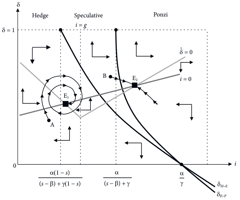
Therefore, as seen by analyzing the figure above, changes in the model parameters can change the economy from a stable situation, such as that existing in the Hedge region, to an unstable region, such as that in the Ponzi region.

6. COMPARATIVE DYNAMICS ANALYSIS

We saw in the previous section that the economic system under study presents, for a significant range of parameters, two possibilities for equilibrium. One of them was included within (or close to) the Hedge region, and the other was included within (or close to) the Ponzi region. As previously mentioned, the nature of the economy’s financial position may change if there are changes in the economy’s key parameters. In fact, we are going to analyze some possibilities for structural change and their consequences for the degree of financial fragility.

Let us start the study with an increase in the banks’ reference level of debt ∆δ->0.⁶ From the following equations, and as illustrated by Figure 3 below, it can be seen that the aforementioned increase moves isoline i =0 upward, while isoline δ =0 remains unchanged.

Source: Authors’ own.

Figure 3 Increase in banks’ reference debt degree 

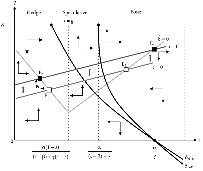
Thus, in the case where the economy is in equilibrium E₁, the relaxation of the debt level perceived as safe by banks causes the economy -if successful in its transition dynamics- to increase its safety margin. Thus, the increase in the banks’ reference level of indebtedness allows for an equilibrium level in the Hedge region with a higher level of indebtedness since the interest rate is lower. In this case, at the new equilibrium point, the level of indebtedness of firms increases at the same time as the system’s security in relation to the possibility of a financial fragility increases.

In contrast, for the case in which the economy is in equilibrium E₂, within or close to the Ponzi region, the increase in the banks’ reference level of indebtedness deepens the financial fragility of the system since the increase in the firms’ indebtedness is accompanied by an increase in interest rates.

Another interesting analysis is the influence of banks’ risk perception, represented by the coefficient θ. As shown in the two equations below, an increase in risk perception by banks has an ambiguous effect on isoline i˙˙=0 (the only isoline affected by such a change).

Thus, the partial derivative of [35] will be positive if and only if sα>ḡs-β+sγi. This will certainly be true if the difference between the propensity to invest in relation to the growth rate of the potential output is positive and, at the same time, if this difference is smaller than the level of the interest rate. Otherwise, the partial derivative of [35] will be negative.

In turn, the partial derivative of [36] will be positive if the level of indebtedness of firms is greater than the level of indebtedness perceived as critical by banks. Otherwise, the partial derivative of [36] will be negative.

Therefore, there are four possible combinations that modify isoline i˙˙=0. By way of illustration, if ∂δ/δθ < 0 and ∂i/∂θ > 0, that is, if the autonomous propensity to invest is not large enough to counteract, for example, the magnitude of the potential product growth rate and, at the same time, if the firms’ degree of indebtedness is greater than that considered critical by banks, then the increase (reduction) in banks’ risk perception will shift the locus downward (upward) i˙˙=0.

Finally, the influence of monetary policy sensitivity can be captured by the following partial derivatives since isoline δ =0 is not affected.

The signs of the partial derivatives are ambiguous. If the level of indebtedness is greater than the level of indebtedness considered critical by banks, then [37] will have a negative sign. Similarly, if the sensitivity of the desired investment in relation to the interest rate is greater than the autonomous propensity to invest, then the sign of [38] will certainly be positive. If this combination occurs, the increase in the sensitivity of the monetary policy will shift isoline i˙˙=0 upward and to the right.

7. FINANCIAL FRAGILITY PROCESS AND COUNTERCYCLICAL POLICIES

Taking the previous discussion as a reference, we can now describe a plausible scenario to highlight the process of financial fragility and outline a possible countercyclical economic policy to combat this process.

In the upward phase of the economic cycle, banks’ risk perception decreases, and the level of firms’ debt assessed as safe by banks decreases. In effect, the increase in the level of debt considered critical moves isoline i˙˙=0 up (and to the left).

When the firms’ effective level of indebtedness is greater than the level of indebtedness perceived as sustainable by banks and the growth rate of potential output is sufficiently greater than the autonomous propensity to invest, the reduction in banks’ risk perception will also move isoline i˙˙=0 up and to the left. In this case, the effect on isoline i˙˙=0 intensifies the relaxation of the critical debt level.

Such a process, as we have seen, and as illustrated in Figure 4 below, will increase the level of indebtedness of firms at the same time as it reduces the interest rate. Consequently, the balance of point E₁ is changed to point E₂. This leads the economy to approach an unstable zone.

Source: Authors’ own.

Figure 4 Countercyclical economic policy 

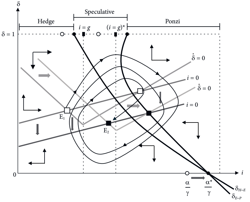
This phenomenon can continue until, eventually (for high levels of debt and low interest rates), it generates a transition dynamic that moves it from the Hedge region to the Speculative region and then to the Ponzi region. Thus, constituting the beginning of the decreasing phase of the cycle or, equally, a period of financial crisis.

In this situation, the movement of the economy occurs through explosive trajectories or alternatively, it finds itself on an unstable equilibrium trajectory of the saddle trajectory type. Regardless of the situation, monetary tightening -by intensifying the sensitivity of the monetary policy- would worsen the state of economic instability, while loose monetary policy could mitigate the crisis by shifting isoline 𝑖 =0 downward and to the right.

The ideal policy, however, would be one that significantly expands the system’s stability zone. A policy of this type can be obtained by increasing the autonomous propensity to invest. This is because the autonomous propensity to invest captures, in the present case, all the determinants of investment that do not depend on the profit rate or the interest rate. For example, an expansionary fiscal policy results from an increase in public investment.

In effect, and as shown in Figure 4, the increase in public sector spending on investment increases the autonomous propensity to invest, which modifies the intercepts of the curves that separate the three debt regimes. Therefore, curves δ_H-E and δ_E-P would move to the right and accentuate their slopes, consequently expanding the Hedge and Speculative regions in comparison to the Ponzi region.

Furthermore, the increase in public investment (autonomous propensity to invest) shifts, as shown in the equations below, from isoline δ˙=0 to the right.

The displacement of isoline δ˙=0 or, equally, of separatrix i = g to the right expands the stable zone of this economy. This, together with the expansionary monetary policy, opens up space for this economy to present a convergent trajectory toward the stable equilibrium point E₁. Finally, it is worth highlighting that this process of convergence to a stable equilibrium will occur through damped spirals. This clearly implies that the adjustment will take place through ups and downs, although these fluctuations decrease over time.

8. FINAL CONSIDERATIONS

By taking into account the cash flow of firms and their accumulation dynamics under the context of endogeneity of the money supply, endogenous monetary policy, and underutilization of productive capacity, it is possible to carry out an analysis of the process of financial fragility along the lines of Minsky.

When it is assumed that banks endogenously supply money and tend to increase their markup rates as a result of the increase in the level of indebtedness of firms vis-à-vis the level of indebtedness perceived as safe, a series of retroactive effects arise that greatly condition the dynamics of financial fragility. These effects become even more complex when considering the presence of a monetary policy via manipulation of the basic interest rate.

In this context, in the short term, there is an inverse relationship between the interest rate and the degree of utilization of productive capacity. This relationship will be more intense the greater the sensitivity of the desired investment to the interest rate and the propensity to invest and the lower the propensity of capitalists (productive and financial) to save, as well as the lower the share of profits in income.

In the long term, the possibility of the existence of multiple equilibria was demonstrated, and a case was illustrated in which there is a stable equilibrium in the Hedge region, characterized by low interest rates and a low degree of debt, and an unstable saddle path trajectory equilibrium in the Ponzi region, characterized by high interest rates and a high degree of debt.

A scenario of financial fragility was outlined in which, in the upward phase of the cycle (recovery and boom period), the perception of risk declines at the same time as the level of debt considered critical by banks is relaxed. As a consequence, the interest rate decreases, and the level of firm debt increases. However, as this happens, the economic system, in its adjustment trajectory, may assume a dynamic that takes it from the Hedge region to the Speculative region and then to the Ponzi region, thus beginning the decreasing phase of the cycle (a period of recession and, eventually, depression).

Faced with a weakening process of this nature, a combination of economic policy based on an expansionary monetary policy and an expansionist fiscal policy embodied in an increase in public investment are outlined. This policy combination has the potential to expand the stable zone, thus opening the possibility for the economic system to assume a dynamic trajectory of convergence to the stable area of the model.