1. INTRODUCTION

^{Benetti et al. (2014}; ²⁰¹⁵⁾ formulated a Classical-inspired temporary disequilibrium model, wherein the economy is monetary and made up of two productive sectors, each branch comprising capitalists who seek to maximize accumulation by investing their earnings in their own sectors. Furthermore, they suppose that monetary prices and exchanges are determined through a market mechanism known as the “Cantillon rule”, and that the monetary system corresponds to one of pure credit, with zero interest rates within each period, along with a simple rule to settle the monetary imbalances that appear during disequilibrium.

Under these assumptions, the authors demonstrate that the dynamics of this economy are non-explosive, which can be convergent to equilibrium or exhibit a limit cycle of order two. Their model is noteworthy for its stability result and, moreover, for its ability to formalize effective disequilibrium positions, primarily due to the Cantillon rule that determines prices and exchanges regardless of the state in which the economy operates. Thus, their model offers greater empirical relevance than the predominant emphasis on equilibrium analyses of nonmonetary economies, commonly observed in mainstream economic frameworks (^{Cartelier, 2018}).

However, besides being unreal and naive, the monetary imbalance settlement rule assumed therein is quite limited since, as its authors demonstrate, it is only applicable to the specific case of a bisector economy with little technical interdependence between sectors. Given that this rule is a non-fundamental hypothesis in the model (justified solely by its simplicity for analyzing economic dynamics), it becomes necessary to consider more realistic and less restrictive alternative hypotheses concerning the monetary system. This would allow us to expand our understanding of the dynamics of market economies under temporary disequilibrium within a Classical theoretical framework.

This paper aims to propose a first alternative model in this direction. Instead of being a pure credit monetary system, the new model will represent a pure cash monetary system. This feature avoids monetary imbalances during disequilibrium, thereby eliminating the need for monetary rules for settlement. The paper will explore the empirical and theoretical relevance of this hypothesis compared to the original model and analyze the stability properties of the equilibrium arising from this new hypothesis.

The document is organized as follows: The next section describes the model proposed by ^{Benetti et al. (2014}; ²⁰¹⁵⁾. Subsequently, the limits of this model are indicated, and the alternative model is presented. Its limits and scope concerning the original model are evaluated, and its statics and dynamics are analyzed. Finally, the conclusions summarize the main results and propose a future research agenda.

2. THE ORIGINAL MODEL

In ^{Benetti et al. (2014}; ²⁰¹⁵⁾ the economy comprises two productive sectors, 1 and 2. Each sector produces one commodity through a single production method with constant returns to scale and using the two goods as circulating capital in fixed proportions represented by the matrix A = [α _ij ] (with i,j = 1,2) where each element α _ij > 0 represents the amount of commodity j that it needs to produce one unit of commodity i. Production takes a single period, and both commodities are perishable.

Labor is implicitly considered in matrix A in the sense that part of each α _ij represents the amount of commodity j that the workers receive in exchange for their labor for producing one unit of commodity i. The real wage is considered constant over time, and it is assumed that there is always an available number of workers that can be employed at this real wage so that the demand for labor is never restricted to that real wage level. Thus, the only agents who make decisions are the capitalists. By hypothesis, it is assumed that they seek to accumulate all their earnings by reinvesting them exclusively in their own productive sector².

On the other hand, the economy operates within a monetary institutional framework of pure credit, in which a public banking institution lends money to the capitalists at the beginning of each period so they can finance their purchases before selling their products. In return, at the end of each period, the capitalists return the same amount of money borrowed (which means that the bank lends money within each period at a null interest rate). In disequilibrium, some capitalists may earn more income than the amount borrowed, while others may earn less, facing challenges in meeting their financial obligations with the bank. ^{Benetti et al. (2014}; ²⁰¹⁵⁾ assume an institutional rule to address these monetary balances, which will be explained later.

Finally, market prices and allocations are determined by the Cantillon rule (^{Benetti, 1996}; ²⁰¹⁹⁾. Under this rule, the monetary price of commodity i (with i = 1,2) is determined by the total amount of money capitalists carry to purchase this commodity divided by the total quantity supplied. And the allocation of commodity i (with i = 1,2) among capitalists is determined by the quantity each capitalist can purchase of i, at its market price, using the amount of money each one proposed to buy this commodity. It is assumed that each capitalist brings to the market the total quantity of the produced good, not just the portion that he plans not to use. Consequently, in each market, a capitalist always participates on both sides -as a buyer and a seller of the same good³.

On the other hand, the money each capitalist borrows from the bank depends on their price expectations. It is assumed that capitalists hold static expectations, so every capitalist believes that prices at time t will equal prices at time t-1. Given that the production technology is also the same among capitalists within each branch (though different between branches), all capitalists within the same branch can be considered in an aggregate manner as being only one capitalist per branch.

The logic of the model is as follows: At the beginning of period t, the capitalist of each branch has the quantity of the good produced with the inputs obtained in the previous period, but which will be offered in the current period and is expressed symbolically as qit-1 (with i = 1,2). Each capitalist aims to accumulate all the income expected from the sale of qit-1 by reinvesting in its own productive branch. With static expectations, the income they expect to receive for qit-1 in t is qit-1pit-1. So this is the amount of money to be borrowed from the bank. With this sum, capitalists of each productive branch want to buy an amount of each commodity that allows them to reach the maximum production level for the next period (that is, to maximize accumulation in the present period). He does not know the actual market prices. Furthermore, to calculate them using the Cantillon rule, it is necessary to determine beforehand the amount of money capitalists will bring to each market. Therefore, each capitalist i (with i = 1,2) must solve the following optimization problem:

Subject to:

Where qie,t is the production level for t that capitalist i aims to maximize -the objective function- at expected prices pit-1 and p2t-1; xi1e,t and xi2e,t are the quantities of commodities 1 and 2 that the capitalists would need as inputs to reach the production level qie,t. To solve this optimization problem characteristic of complementary goods, one must consider that the solution has to always satisfy the following condition⁴:

Substituting equation [3] into equation [2], we determine the input demands for commodities 1 and 2 at expected prices p1t-1 and p2t-1:

And substituting equation [4] and equation [5] into equation [1], we determine the expected level of production:

To that end, each capitalist will lead to the market for commodity 1 the amount of money mi1t=xi1e,tpit-1=αi1pit-1qie,t and the amount mi2t=xi2e,tp2t-1=αi2p2t-1qie,t to the market for commodity 2, in an attempt to purchase xi1e,t and xi2e,t respectively.

With the amounts of money that each capitalist brings to the market for i and the amount qit-1 that the capitalist of branch i brings to the market, Cantillon’s rule determines the monetary price of i as follows:

And the allocations of commodity i that obtains capitalist of branch j is determined as follows:

Note that xjit=xjie,t only when capitalists correctly anticipate the price of that commodity (pit=pit). In any other case, the capitalist j obtains a different quantity from what was initially anticipated at expected prices from the market. Particularly, if pit<pit, then xjit>xjie,t, meaning that capitalist j purchases more than initially intended at the expected price. As ^{Benetti et al. (2014, p. 530)} argue, this case does not violate the voluntary exchange principle (^{Bénassy, 1986}) because xjie,t is the amount of i that capitalist j wanted to buy at expected prices before knowing market prices. And once he knows market prices, he doesn’t know yet if he has obtained more or less of i than what he wants because, as will be seen below, the final allocations that each capitalist will obtain will differ from the market allocations due to the institutional rule of balance settlement.

Once market prices and allocations are determined, the expenses and income received by the capitalists can be calculated. According to Cantillon’s rule, capitalists always spend the amount of money they bring to market, so the expense that each capitalist i does is: qit-1pit-1=miit+mijt (with i = 1,2). And capitalists always sell all the amount of the commodity they bring to the market, so the income that each capitalist i receives is: qit-1pit=miit+mjit. Note that only when capitalists correctly anticipate the price of the commodity they produce (pit=pit-1), their expenses equal their income, and they have no problem meeting their obligations to the bank at the end of the period. In other cases, their expenses will differ from their income and if the former outnumber the latter, the capitalists will not be able to repay their loan to the bank. However, the sum of the money balances between capitalists always equals zero. To see this, let’s call Sit and S2t the money balances of capitalist 1 and 2, respectively, and sum them:

So always:

The last equation implies two things: Firstly, if one capitalist has a positive money imbalance, the other will have a negative one. Secondly, the money that the latter lacks to pay his debt to the bank is of the same magnitude as the amount of money that the former has left over after paying its debt to the bank. Thus, ^{Benetti et al. (2014}; ²⁰¹⁵⁾ assume the following institutional rule to solve these monetary imbalances: The capitalist with a positive imbalance gives his surplus to the capitalist with a negative imbalance in exchange for a basket of commodities, whose physical composition is chosen by the first one and whose value at market prices is equal to the monetary imbalance.

To illustrate this rule, suppose that, at the date t, capitalist 1 is in surplus and capitalist 2 is in deficit. How will the former choose his basket? He will select the one that enables him to fulfill the requirements necessary for accumulating all his income at market prices. To calculate those amounts, he must solve the optimization problem described in equations [1], [2], and [3] but now considering market prices as parameters (instead of the expected ones), leading to the following results:

Where q1t is the level of production that capitalist 1 will reach and x1if,t (with i=1,2) is the final allocation of commodities that capitalist 1 will have (and will use to produce q1t for the next period). Therefore, capitalist 1 requests capitalist 2 for the amounts α11q1t-x11t of commodity 1 and α12q1t-x12t of commodity 2. Capitalist 2 will be left with x21f,t=q1t-1-α11q1t of commodity 1 and x22f,t=q2t-1-α12q1t of commodity 2. So, capitalist 1 will be able to accumulate all of the income obtained in the market, which will allow him to produce q1t for the next period, and capitalist 2 will only be able to accumulate the commodities that enable him to reach the following level of production for the next period:

The remaining commodities that cannot be accumulated by capitalist 2 will be unproductively consumed by himself (bearing in mind that both commodities are perishable).

This rule might be unfeasible in some instances where the excess demand of the capitalist with a monetary surplus (capitalist 1 in the illustration) for a particular commodity is equal to or exceeds the availability of that commodity, which, in turn, belongs to the capitalist with the monetary deficit (capitalist 2 in the illustration). In such situations, if capitalist 1 acquires all the available quantity of that commodity from capitalist 2, the latter’s reproduction would be at risk, posing a threat to the reproduction of the entire economy.

^{Benetti et al. 2014} demonstrate that a sufficient condition to avoid this problem, ensuring the rule is always viable regardless of the initial conditions, is that the determinant (D) of A meets the following property:

This property implies that α₁₂ α₂₁ < 17.9444 a₁₁ a₂₂ and, economically, it means that the productive interdependence between industries (expressed in the multiplication of α₁₂ and α₂₁ parameters) is not so significant compared to the productive dependence within the industry (described in the multiplication of α₁₁ and α₂₂ parameters). In particular, the first one must be at least 17.944 times less significant than the last one.

^{Benetti et al. (2014}; ²⁰¹⁵⁾ assumed that equation [14] is fulfilled and analyzed the properties that arise in the dynamics of the economy under these hypotheses. Their most significant result demonstrates that this economy exhibits a non-explosive dynamic, characterized by the following particularities: “If D is positive, the system converges towards a von Neumann growth path. If D is negative, either that convergence is local (and maybe global), or there exists a limit cycle of order two, depending on the ratio between the second and the first (or dominant) eigenvalue of matrix A” (^{Benetti et al., 2014, pp. 533-534}). In the next section, the model formulated by ^{Benetti et al. (2014}; ²⁰¹⁵⁾ will be criticized, and an alternative model will be proposed.

3. THE ALTERNATIVE MODEL

The ^{Benetti et al. (2014}; ²⁰¹⁵⁾ model is interesting because it constitutes an alternative to most of the classical gravitation models (^{Caminati, 1990}; ^{Bellino, 2012}; ^{Bellino and Serrano, 2018})⁵ since, unlike those models, in that one there is no capital mobility between branches, the dynamic is effective (or not virtual), and prices and allocations are always perfectly determined regardless of the state in which the economy operates.

However, ^{Benetti et al. (2014}; ²⁰¹⁵⁾ model has an important problem regarding its monetary balance settlement rule because, besides being unreal and naive, it is very restrictive in two different ways. Firstly, its viability can only be assured (regardless of the initial data) when condition [14] holds. However, this condition is quite stringent for a market society characterized by a prevailing social division of labor, as it would be expected that inter-industrial dependence is significantly greater than intra-industrial dependence in such societies.

Secondly, it is also excessively restrictive because it can only be used when the economy is bi-sectoral. In an n-sectoral economy with n > 2, the accumulation plans of the capitalists with a monetary surplus in some date may not be in general compatible with the availability of commodities that the capitalists with monetary deficits have. So, it would be necessary to specify what happens with this rule in such cases (a problem that resembles the neoclassical question of the theory of value of making individual plans compatible through general equilibrium prices, which allows us to foresee that a rule for such cases would eventually be quite complex).

So, how can we replace this hypothesis? There are likely several alternative rules to the one used by ^{Benetti et al. (2014}; ²⁰¹⁵⁾. In this paper we choose to adopt a monetary system radically opposed to the one assumed by ^{Benetti et al. (2014}; ²⁰¹⁵⁾ that holds a privileged place in the history of monetary theory: We will assume a pure cash monetary system. In this system, credit is excluded, ensuring there are never any monetary balances in the economy since, by definition, individuals cannot spend more money than the amount they already have in their pockets.

This system is important in monetary theory because, at least since ^{Wicksell (1936)}, it is regarded, along with the pure credit system, as one of the two extremely opposite cases in whose lineal combination any contemporary monetary system is found⁶. On the other hand, while this pure cash monetary system may be considered equally unrealistic as the pure credit monetary system with zero interest rate and the simple imbalance settlement rule proposed by ^{Benetti et al. (2014}; ²⁰¹⁵⁾, there is a crucial distinction. A pure cash monetary system might exist in small market economies where financial systems are not well-developed (^{Fauvelle, 2024}). In contrast, it is unlikely that there will ever be a pure credit monetary economy with zero interest rate and such straightforward rules for settling monetary imbalances.

So, let us formalize the new monetary hypothesis. It will be assumed that the economy operates in a monetary institutional framework of metallic money. That is, it will be assumed that there is a third object in the economy -let’s call it “gold”- that does not enter as an input in any productive branch nor as a consumption for the workers. Instead, it only serves as money in its three functions (medium of exchange, unit of account, and store of value). It is assumed that there is no form of credit and that the amount of gold in the economy and its legal price are constant over time. Thus, capitalists can only modify their initial endowment of money by purchasing and selling commodities, complying with the cash-in-advance constraint (^{Clower, 1967}).

Since, by the Cantillon rule, capitalists always spend all the money they carry and always sell all the commodities they offer in the market, the amount of money that each capitalist will have at the beginning of any period t will be equal to the value of the amount of commodity they sold in t-1, that is: q1t-2p1t-1 (with i = 1,2). It is assumed that both markets for commodities operate simultaneously, implying that capitalists’ expenditures can only be financed with the money carried forward from the previous period (the cash-in-advance constraint), not with funds acquired from the current sale of their products.

As a result, the decision problem capitalists face in allocating their money to buy goods in both markets remains akin to the original model. The only difference lies in the budget constraint, which is now constrained by the amount of money obtained in the previous period (q1t-2p1t-1), rather than being restricted by the amount of money borrowed (q1t-1p1t-1). Mathematically:

Subject to:

Which leads to:

and

Each capitalist will lead to the market of 1 the amount of money mi1t=xi1e,tp1t-1=αi1p1t-1qie,t and the amount mi2t=xi2e,tp2t-1=αi2p2t-1qie,t to the market 2, to try to buy xi1e,t and xi2e,t respectively. And the price and the commodities allocations determined by the Cantillon rule will be:

Due to the absence of credit in this model, the quantity xjit they have purchased in each market will represent their final market allocations. Consequently, the level of production they will achieve for the next period will be:

Once each branch’s absolute production levels and the monetary prices of each good have been determined, it is possible to determine their relative values. Thus, for example, the relative price of period t is equal to:

Where pt-1=P1t-1P2t-1, qt-1=q1t-1q2t-1 and qe,t=q1e,tq2e,t. This last variable being equal to:

So, replacing equation [24] by equation [25], we have:

Regarding production, even though, in absolute terms, the level of each branch depends on a ‘min function’ (equations [22] and [23]), in relative terms, it will always be equal to the relative structure of the desired production level (equation [25]). The reason for this is that, given that both capitalists share the same price expectations, the maximum production level each can achieve, with the allocations obtained in the market and based on their respective techniques, is uniformly restricted for the same good. This restriction occurs because the imbalance in the assignments affects them in the same way.

To illustrate this, suppose that P1t-1/P1t<P2t-1/P2t. Then by equation [21], we will have x11t/α11<x12t/α12 and x21t/α21<x22t/α22. This implies that the maximum level of production that both branches can achieve, given their techniques, is restricted by the allocation of the same good (in this case by good 1 and, if P1t-1/P1t>P2t-1/P2t, by good 2). Now, in relative terms, this implies that the productive structure always turns out to be the same as the desired one because, according to equation [21], for any of the previous cases it is true that:

So, it is always true that q ^t = q ^e,t . In this way, according to equation [25], the relative structure of the effective product is equal to:

This implies that the ‘min function’ disappears to determine the relative values of the quantities produced. Thus, equations [26] and [28] compose the system of difference equations that synthesize the dynamics of the economy. Since the dynamic equilibrium consists of a vector of relative prices, p*, and a productive structure, q*, such that …= p ^t-1 = p ^t = p ^t+1 = … and …= q ^t-1 = q ^t = q ^t+1 = …, replacing p ^t and p ^t-1 by p* and q ^t , q ^t-1 and q ^t-2 by q* in equations [26] and [28] we can find the equilibrium values of relative prices and the productive structure. These values are equal to the column and row eigenvector associated with the dominant eigenvalue of matrix A of productive coefficients, i.e. the Classical price of production and equilibrium quantities. In the case of equilibrium relative prices:

Thus, the equilibrium of this economy is the same as that of ^{Benetti et al. (2014}; ²⁰¹⁵⁾. On the other hand, the system of equations [26] and [28] is nonlinear of second degree. To analyze its properties of local asymptotic convergence to equilibrium, that is, to know under what conditions any trajectory that starts from a point sufficiently close to equilibrium converges to it, as time progresses, this system can be transformed into a first-degree system by introducing a new variable, z ^t-1 , defined as follows: z ^t-1 = q ^t-2 , and making a linear approximation of this system. With z ^t-1 the original system becomes:

The linear approximation of this system is obtained by applying the Jacobian, J, defined as:

Each component is the partial derivative of each of the three equations for each of the three variables evaluated at the equilibrium point, that is, evaluating p ^t-1 as p*, q ^t-1 as q*, and z ^t-1 as q*. The resulting matrix J is equal to:

Where

and

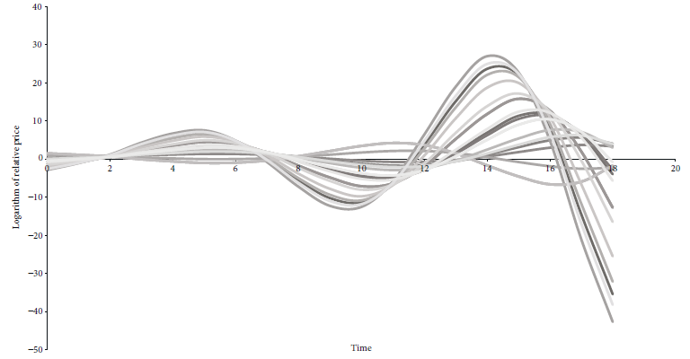
To analyze the local stability of this system, we evaluate the determinants of this system. Surprisingly, this value is equal to ( J (= -1, implying, according to ^{Gandolfo (1997, pp. 117, condition X}), that the equilibrium is locally unstable. This means that small perturbations from the equilibrium point lead to trajectories that move away. On the other hand, numerical simulations show that this equilibrium is also globally unstable, which means that the economy will have the same unstable pattern independent of the distance to the equilibrium at which the initial point begins. This property can be verified graphically in Figure 1, which shows the dynamics of the logarithm of the relative price (the logarithm was applied to p _t to smooth and homogenize the scale in which this variable varies over time), which results from running twenty simulations using the parameters: α₁₁ = 0.54, α₁₂ = 0.46, α₂₁ = 0.6, α₂₂ = 0.2 for twenty different initial conditions of the values p ^t=0 , q ^t=0 and q ^t=-1 , randomly determined.

Thus, unlike the ^{Benetti et al. (2014}; ²⁰¹⁵⁾ model, the economy tends towards crisis in the alternative model, so government intervention is justified to set the equilibrium values to avoid economic crisis. In this regard, it is interesting to see how variations in the monetary system have such an important impact on the dynamic stability properties of the economy. And considering that the pure cash monetary system hypothesis is more relevant⁷ and less restrictive⁸ than the monetary hypothesis assumed in the ^{Benetti et al. (2014}; ²⁰¹⁵⁾ model, the result of the instability of the alternative model with respect to the original one stands out even more.

4. CONCLUSIONS

In this study, we have demonstrated that the dynamics of a bisector economy with a pure cash monetary system, wherein capitalists accumulate all profits and prices are determined by the Cantillon rule, is locally (and by mean of simulations globally) explosive, suggesting that the economy, if initially in disequilibrium, drifts further away from equilibrium, leading to a potential economic crisis. Consequently, government intervention is justified in this kind of economy to avoid a crisis.

This result contrasts with the stability of the original model by ^{Benetti et al. (2014}; ²⁰¹⁵⁾, which, however, is less relevant and more restrictive than the model proposed in this study. Nevertheless, it is essential to acknowledge that while theoretically interesting, a pure cash monetary system remains a hypothesis far removed from reality. Considering the complex financial systems characterizing contemporary capitalist economies, there is still a considerable distance to cover in the research program on temporal disequilibrium under a Classical approach. Future research efforts could involve formulating alternative models with more realistic hypotheses about the monetary system. For instance, exploring monetary credit systems, with non-zero interest rates and incorporating more realistic settlement rules for monetary imbalances, could provide a nuanced perspective on the dynamics of market economies under temporary disequilibrium within the Classical theoretical framework.