


 nueva página del texto (beta)
 Inglés (pdf)
 Artículo en XML
 Referencias del artículo
 Enviar artículo por email
 Citado por SciELO
  Similares en
SciELO
Similares en
SciELO 
 Permalink
1. INTRODUCTION
Barred spiral galaxies are one of the most intriguing kind of objects in the universe. In these galaxies, a large bisymmetrical structure grows in the center of the disk component, modifying drastically the kinematics and the dynamics of the barions contained in the central part of the galaxy. Dark matter is also influenced by the formation of the bar structure (Valenzuela & Klypin 2003).
For decades, barred galaxies have been the subject of several observational, theoretical and numerical studies. It is now well established that bars significantly influence their host galaxies in various ways. As the bar grows over time, it transfers angular momentum from the inner disk to the outer disk and the dark matter halo, as discussed by several authors (Lynden-Bell & Kalnajs 1972; Sellwood 1981; Athanassoula 2003; Athanassoula et al. 2013). The growing bar will also direct gas to the center of the galaxy along the narrow lanes that represent loci of shocks within the bar region (Sorensen et al. 1976; Athanassoula 1992; Davoust & Contini 2004; Villa-Vargas et al. 2010; Spinoso et al. 2017; George et al. 2019) triggering the nuclear activity. The influence of the bar on gas dynamics has been the subject of extensive research over the years, with a wide range of studies dedicated to this topic (e.g. van Albada & Roberts 1981; Schwarz 1985; Piner et al. 1995; Maciejewski et al. 2002; Kim & Stone 2012; Pastras et al. 2022; Romeo et al. 2023; Sormani et al. 2024 and references therein).
There are also studies proving the kinematics of bars to be significant. In numerical simulations, the bar pattern speed (Ω B ), or angular velocity of the bar, is closely linked to the evolution of both the bar and its host galaxy. As the bar grows and transfers angular momentum to its surroundings, it generally slows down, resulting in a decrease in the pattern speed (Debattista & Sellwood 2000; Athanassoula 2003; Martinez-Valpuesta et al. 2006; Okamoto et al. 2015; Wu et al. 2018). The bar evolution is also influenced by its surrounding environment. Recent studies have demonstrated that the angular momentum of the dark matter halo plays a crucial role in shaping the evolution of both the bar and the disk, impacting the bar pattern speed, instability timescales, and other dynamics (Saha & Naab 2013; Petersen et al. 2016; Collier et al. 2018; Collier & Madigan 2021).
Observational studies have shown that barred galaxies exhibit increased star formation in their central regions (Matsuda & Nelson 1977; Hawarden et al. 1986; Garcia-Barreto et al. 1991; Kenney et al. 1992; Alonso-Herrero & Knapen 2001; Hunt et al. 2008; Coelho & Gadotti 2011; Ellison et al. 2011; Lin et al. 2020; Géron et al. 2024) as well as in the bar-end regions (Reynaud & Downes 1998; Verley et al. 2007; Díaz-García et al. 2020; Fraser-McKelvie et al. 2020; Maeda et al. 2020; Géron et al. 2024). Conversely, star formation is suppressed along the arms of the bar (Reynaud & Downes 1998; Zurita et al. 2004; Watanabe et al. 2011; Haywood et al. 2016; Géron et al. 2024). These observational and numerical studies highlight the significant role that bars play in the evolution of their host galaxies.
In this paper, we present a new numerical investigation by studying a large number of three-dimensional response models. The axisymmetric part of the models is generated to fit the Galactic circular rotation curve proposed by Sofue (2020). We tested a number of parameters such as disk particles velocity dispersion, and mass, size and angular pattern speed of the imposed bar. In § 2 we present our models, parameters, initial conditions and orbit integrations, and in § 3 we discuss the resulting bar structure observed in the particle distributions. The resulting values are discussed in § 4 and, finally, in § 5 we present a general discussion and our conclusions.
2. SIMULATIONS
2.1. Galactic Models
The selected gravitational potentials are composed by a sum of the axisymmetric and bar components. The axisymmetric component itself is a superposition of several elements: a core and a bulge, both modeled by a Plummer potential (Plummer 1911), a disk represented by a Miyamoto-Nagai model (Miyamoto & Nagai 1975), and a halo described by a logarithmic potential (Richstone 1980). The full axisymmetric potential is then
where r 2 = x 2 + y 2 + z 2, while R 2 = x 2 + y 2. M c1 and M c2 are the masses of the bulge and the core, respectively, and r c1 and r c2 are their radial scale lengths. M D is the disk mass and a and b its structural parameters. For the halo, v H is the asymptotic velocity and r H its radial scale length. By comparing the circular velocity profiles obtained from different parameter sets with the observed velocities in the Milky Way within the first 40 kpc, as reported by Sofue (2020), and by employing the gradient descent method, we identified three parameter sets with nearly identical χ 2 values. This indicates that the potentials corresponding to these parameters are degenerate. However, these potentials exhibit distinct characteristics from one another. Figure 1 displays the circular velocities derived from the three models, which we will henceforth refer to as Model 1 (left panel), Model 2 (middle panel), and Model 3 (right panel), based on the influence of their respective disks. The parameter values corresponding to each model are provided in Table 1.
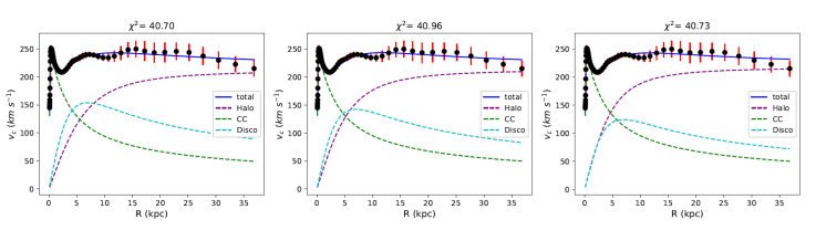
Fig. 1 The circular velocity curves corresponding to the axisymmetric potential for three different sets of parameter values. CC means Central Component (bulge+core). These curves are compared with the circular velocity of the Milky Way (Sofue 2020) within the first 40 kpc, along with their associated χ 2. The color figure can be viewed online.
TABLE 1 PARAMETERS FOR THE AXISYMMETRIC MODELS
| Model | rc1 (kpc) | Mc1 (M⊙) | rc2 (kpc) | Mc2 (M⊙) | a (kpc) | b (kpc) | MD (M⊙) | rH (kpc) | vH (km/s) |
|---|---|---|---|---|---|---|---|---|---|
| 1 | 1.46 | 1.07 × 10¹⁰ | 0.278 | 1.01 × 10¹⁰ | 4.66 | 0.233 | 6.99 × 10¹⁰ | 7.68 | 212 |
| 2 | 1.46 | 1.15 × 10¹⁰ | 0.275 | 1.00 × 10¹⁰ | 4.72 | 0.236 | 6.06 ×10¹⁰ | 6.78 | 213 |
| 3 | 1.45 | 1.16 × 10¹⁰ | 0.274 | 9.96 × 10⁹ | 4.69 | 0.235 | 4.60 × 10¹⁰ | 5.73 | 217 |
2.2. Bar Models
For the bar component, we employed the ellipsoidal Ferrers potential. The mass density associated with this potential is defined as:
where
To simplify the models, we fixed the ratios between the semi-axes, setting b B = a B /3 and c B = a B /6. However, the major semi-axis a B was varied, considering three distinct values: 6, 4.5, and 3 kpc. We introduced the bar component as a smooth time-dependent function by gradually transferring mass from the disk to the bar in the following way:
Here,
The parameter
We are now able to analyze the bar rotation rate in a two-dimensional parameter space for ℛ corresponding to each axisymmetric model, along-side the three selected values for the bar length, as illustrated in Figure 2 for Model 1. This methodology allows for the identification of models featuring either fast or slow bars, with varying values of μ B and Ω B . Therefore, we focused on models with μ B = 0.1, 0.2, 0.3, 0.4, 0.5 and Ω B = 20, 25, 30, 35, 40, 50, 60 km/s: Furthermore, only models with 1 ≤ ℛ ≤ 3 were analyzed (indicated by red dots in Figure 2), corresponding to bars classified as fast and slow by Aguerri et al. (2015).
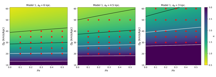
Fig. 2 Parameter space for ℛ with respect to the parameters μ B and Ω B for model 1 and three values of bar length. The red dots are the models we studied in this article. Here we show the values only for Model 1, because there is no significant change of ℛ when considering the three axisymmetric models (Model 1, Model 2 and Model 3), once they are time independent (see text). From bottom to top, the straight lines in each plot denote equal ℛ: 3 and 2 (white solid lines) and 1.4 and 1 (black solid lines). The color figure can be viewed online.
2.3. Initial Conditions and Orbit Integrations
Given our focus on stars within the disk, we selected the initial positions of the test particles following the axisymmetric distribution of the Kuzmin model whose surface density is (Binney & Tremaine 2008):
We have chosen to use KT models to create the initial particle distribution since our Miyamoto-Nagai models have a scale length ratio (a/b) of 20, i.e. the disks are very thin. Furthermore, all the particles are initially in the galactic plane (z(t = 0) = 0). Considering the relationship between surface density and the number of stars, we observe that at a given radius, the number of stars can be expressed as N K (R) = 2πΣ K (R). By employing the Monte Carlo method, we can achieve a well-distributed arrangement of stars within the galactic plane. The maximum radius selected was given by R max = 1.5R CR . Although all particles are initially positioned within the galactic plane, the three-dimensional aspect of the simulations is established through the introduction of an initial velocity component along the z-axis.
For the velocity initial conditions, we decided to make
where σ R , σ T and σ z are the radial, tangential and vertical velocity dispersions, σ R (0), σ T (0) σ z (0) are their central values, and h R , h T and h z are the scale lengths. In their work, Lewis & Freeman (1989) computed the specific values of h R and h T for the Milky Way, which were found to be 4.37 kpc and 3.36 kpc, respectively. In the same work, Lewis and Freeman also assumed that the ratio of radial velocity dispersion σ R to vertical velocity dispersion σ z remains constant. Consequently, we have chosen h z = h R .
For our research, we have chosen to equate the three central velocity dispersions (σ R (0) = σ T (0) = σ z (0) = σ D ). Additionally, we explore three distinct values for this new parameter: 100, 80 and 50 km/s.
Hence, in total, we have 5 different galactic parameters: three different axisymmetric models, five distinct bar/disk mass ratios, seven angular velocities, three sets of bar lengths and three disk central velocity dispersion. This resulted in 945 different models. However, as mentioned before, only models with 1 ≤ ℛ ≤3 were studied, and then our - final set of simulations discussed here included 708 simulations. Each simulation comprised a total of 30,000 test particles, yielding a total of 21,240,000 calculated orbits. A concise summary of the model parameter space is presented in Table 2.
TABLE 2 MODELS PARAMETER SPACE
| Parameter | Value |
|---|---|
| Model | 1, 2, 3 |
| σ D (km/s) | 50, 80, 100 |
| a B (kpc) a | 3, 4.5, 6 |
| μ B | 0.1, 0.2, 0.3, 0.4, 0.5 |
| Ω B (km/s/kpc) | 20, 25, 30, 35, 40, 50, 60 |
a The axis ratios are b B = a B /3 and c B = a B /6.
The integration was carried out using a fourth-order Runge-Kutta integrator, employing Fortran subroutines. To assess stability, we monitored the Jacobi energy of test particles following bar growth. Typically, ΔE J is better than 10-10 for t > T max , since only then the models become time independent. The total simulation time was 11.25 Gyr, during which 1225 snapshots were captured at equidistant intervals. The bar mass growth ceases at T max = 1 Gyr to ensure 1024 snapshots after the bar mass evolution. This number of points (210) was chosen to simplify the Fast Fourier Transform analysis.
3. ESTIMATING PROPERTIES OF THE BAR
3.1. Detecting the Periodic Orbits x 1 and x 2
As highlighted by several authors (e.g., Contopoulos (1970), Athanassoula et al. (1983), Sellwood & Wilkinson (1993), Skokos et al. (2002a) and Patsis & Athanassoula (2019), periodic orbits play a crucial role in shaping the structure of barred galaxies. These periodic orbits are categorized into four primary families, namely the x 1, x 2, x 3 and x 4 family orbits, following the classification by Contopoulos & Papayannopoulos (1980), with the most significant being the x 1 and x 2 families. Identifying these periodic orbits is essential for understanding the dynamics of barred galaxies.
To detect these orbits in our simulations, we applied a Fourier transform on the particle coordinates projected onto the equatorial plane: x(t), y(t), and R’(t) = R(t) -
It is crucial to emphasize that this analysis was conducted after the bar has reached its final mass, i.e., for t > T max , as in our approach the stellar orbits stabilize and maintain a consistent pattern after the bar growth. In addition, prior to performing the Fourier transform, we applied a Hanning window function to the orbit positions. The purpose of this window function was to mitigate signal ‘leakage’ in the Fourier spectra.
We can now identify sticky orbits around the x 1 and x 2 families of periodic orbits (Contopoulos & Harsoula 2008; Katsanikas et al. 2013), but for simplicity, we will refer to them as members of the x 1 or x 2 families. An orbit is classified as part of the x 1 family if it satisfies the condition 1.9 ≤ ω R /ω x ≤ 2.1 and A x /A y ≥ 2. On the other hand, orbits that meet the criteria 1.9 ≤ ω R /ω x ≤ 2.1 and A x /A y ≤ 0.5 are associated with either the x 2 or x 3 family. However, it is important to note that the x 3 family is significantly less stable than the x 2 family (Skokos et al. 2002b), and as such, the presence of sticky-chaotic orbits around x 3 is expected to be minimal, making them insignificant for classification purposes.
Having identified the orbits belonging to the x
1 and x
2 families, we can now quantify the number of orbits in each family, denoted as
3.2. Bar Strength
We also performed a Fourier analysis on the stars positions to calculate the bar strength. For this, we computed the m = 2 mode Fourier coefficients (a 2 and b 2) based on the particle positions located within an annulus of width ΔR at a radius R. Hence, as highlighted by Chantavat et al. (2024), the amplitude of the bar is:
where the bar strength corresponds to the maximum value à 2 within R CR , expressed as:
We applied this method to each snapshot, making A 2 a time-dependent parameter A 2(t). This time evolution of A 2(t) was then used to analyze the properties and dynamics of the orbits in our galaxy models. In Figure 3, we observe the temporal evolution of A 2(t) for two given simulations. In the same figure, a smoothed version of this quantity is shown (the smoothing process employed a Savitzky-Golay filter with a sixth-order polynomial).
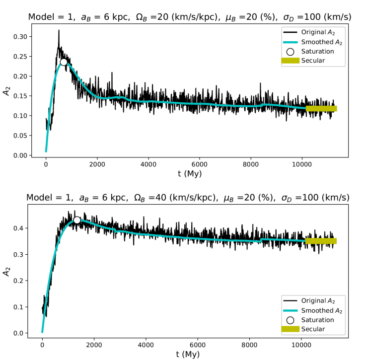
Fig. 3 Evolution of the bar strength A 2(t) over time (black line) for two different models. The cyan line corresponds to the smoothed versions. Additionally, the white/black dot indicates the point of saturation in A2(t), while the horizontal yellow line represents the secular value associated. Notice the different behavior of A 2(t); in one simulation, A 2(t) decreases after the time of saturation, while in the other model, A 2(t) remains more or less constant. The color figure can be viewed online.
Even with the smoothed curves of A 2(t), analyzing each curve individually is impractical since we have a very large number of galaxy models; therefore, we seek for characteristic values that help us to evaluate the model.
One such value is the saturation point in A 2(t). As observed in Figure 3, the A 2(t) curves initially experience a rapid growth, followed by a decline. Notably, several curves exhibit this decline after a specific time. We designate the values at this inflection point as A sat and t sat .
Another characteristic value becomes evident toward the end of the simulations for A 2(t). At this point, the curves exhibit minimal changes over time. This behavior is expected since the structure of rotating Ferrers bars is primarily supported by the stable portion of the x 1 family. In a response model, any changes in A 2 after a couple of bar revolutions beyond T max can therefore be attributed to the influence of chaotic or escaping orbits. To quantify this stability in the A 2 values, we calculated the average values over the last 1 Gyr. specifically, we denote these values as < A sec >.
An additional observation is the difference between A sat and < A sec >. Consequently, we designate this difference as another characteristic value, denoted by ΔA = A sat - < A sec >.
4. FEATURE PARAMETERS VS RESULT VALUES
Having obtained several parameters that characterize the orbital behavior in each galaxy model, namely:
We employed two methods to compare the result values and the feature parameters. The first method involves calculating Spearman correlation coefficients (Spearman 1904), which measure the strength and direction of a monotonic relationship between two ranked variables. This approach allows us to observe how the feature parameters affect the result values. The coefficients, along with their corresponding p-values (which represent the probability of obtaining test results at least as extreme as the result actually observed (Spearman 1904)) are presented in Figure 4.
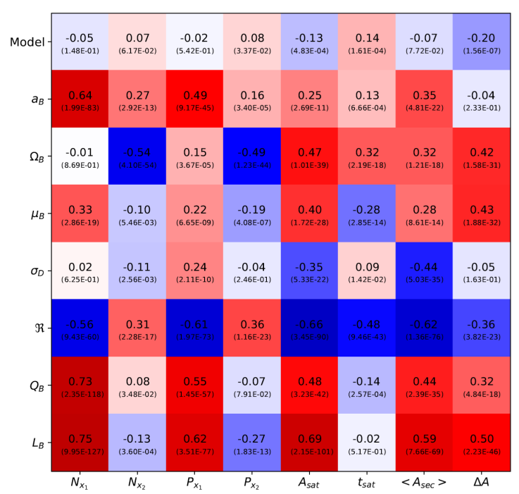
Fig. 4 Spearman correlation coefficients between the result values and the feature parameters for all of our models (708 models). The associated p-values are provided in parentheses. Bright red colors represent high correlations, while bright blue ones represent high anti-correlations. The lighter the color, the weaker the correlation of a given feature parameter with the result value.
The second method, derived from machine learning, uses the permutation feature importance within a Random Forest Regressor (RFR). An RFR (Breiman 2001) is an ensemble learning method that combines multiple decision trees to improve predictive performance and reduce overfitting.
Initially applied in this field by Garma-Oehmichen et al. (2021), this approach evaluates the contribution of each feature to a given result value by randomly shuffling the values of a specific feature and measuring the resulting change in the so called R
2 score. The R
2 score quantifies how well the model explains the variance in the result value, ranging from 1 (perfect fit) to -∞ (arbitrarily poor t) (Pedregosa et al. 2011). The difference between the R2 score for the original data (
We trained the RFRs using 80% of the data, reserving the remaining 20% for testing, to nd the optimal number of features for each result value. We set the number of trees in the model to 1,000 and determined the optimal model by selecting the one with the highest R 2. After identifying the best parameters for each result value, we retrained the models using the entire data set, following the method proposed by Garma-Oehmichen et al. (2021).
Finally, we estimated the permutation feature importance after 1,000 permutations for all result values, with the outcomes illustrated in Figures 5 and 6, along with the feature parameter distributions. It is crucial to emphasize that the importance values, represented by
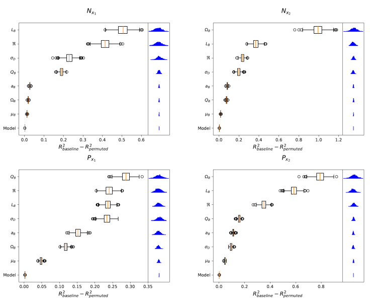
Fig. 5 The permutation feature importance calculated using RFRs, trained to predict each specific result value related to thex
1 andx
2 families, is depicted. Each feature was permuted 1000 times, generating a distribution of
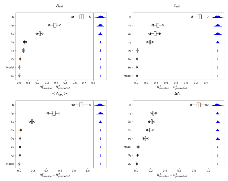
As previously noted, we are now able to assess the relative importance of each feature parameter for a given result value through the use of feature importance, as illustrated in Figures 5 and 6. Additionally, the Spearman correlation coefficients presented in Figure 4 provide insights into the nature and direction of the relationships between feature parameters and result values. By combining these two methods, we have uncovered notable findings, which will be explored in detail in the following section.
5. DISCUSSION AND CONCLUSIONS
From the results presented in Figures 4, 5 and 6 we can derive numerous insights for each result value (
5.1. Evolution of x 1 and x 2 Orbits and Double Barred Galaxies
It is essential to note that the methods introduced in § 4 are directly applied to the response model, allowing for the tracking of changes introduced whenever the parameter combinations depicted in Figure 4 occur. This approach provides significant practical value in the analysis of fully self-consistent N-body models, enabling a comprehensive assessment of the evolution of key orbital structures, particularly the x 1 and x 2 families.
In Figure 5, it is evident that the ℛ parameter is the second most influential feature for determining
Previous studies using N-body simulations (e.g., Athanassoula 2003; Manos & Machado 2014) have demonstrated that in barred galaxies, Ω B tends to decrease over time, consequently ℛ increases. When combined with our findings, this suggests that barred galaxies may initially feature a fast bar, characterized by a high number of x 1 orbits, and gradually lose some of these orbits as the system evolves. Simultaneously, as Ω B decreases, the bar could be acquiring a larger number of x 2 orbits.
Moreover, the presence of a significant concentration of x 2 orbits could offer an explanation for the existence of a secondary bar in certain galaxies (Friedli et al. 1996; Maciejewski et al. 2002; Erwin 2004; Wozniak 2015; Erwin 2024). This indicates that double-barred galaxies may be dynamically more evolved systems.
5.2. Characterizing Bar Strength Evolution Through ΔA
Figure 3 presents two distinct bar strength curves over time, A 2(t). The first curve exhibits rapid growth until it reaches a saturation point. After saturation, the bar rapidly weakens until it reaches an equilibrium (as expected for response models) with < A sec >. In contrast, in the second curve the bar also weakens beyond the saturation point, although at a much slower rate. Looking at the other A(t) curves we can note that there are intermediate cases.
The parameter ΔA plays a crucial role in understanding this behavior. A large positive value of ΔA indicates that A sat is larger than < A sec >, aligning with the behavior observed in the first case in Figure 3. Conversely, a small ΔA corresponds to a behavior more related to the second case shown in the same figure.
As previously discussed, thex 1 family of orbits forms the backbone of rotating Ferrers bars, remaining stable in the region that supports the bar. In a response model, the decreasing of ΔAcould be attributed to the presence of chaotic or escape orbits within the system. To verify this last statement, a study using an index to quantify the chaotic behavior of the orbits as GALI2 (Skokos et al. 2007; Chaves-Velasquez et al. 2017; Caritá et al. 2019) could be performed. However, this is beyond the scope of the present paper.
The permutation feature importance analysis for ΔA(Figure 6) shows that the primary feature parameter, with a significantly larger importance compared to other feature parameters, is ℛ. Furthermore, the Spearman correlation between ΔAand ℛ (as shown in Figure 4) is negative. From this, we can infer the following:
Slow Bars: In cases of slow bars, the models losex 1 particles at a very slow rate after reaching the saturation point (as in the second case mentioned earlier in Figure 3).
Fast Bars: Conversely, fast bars experience fast particle loss beyond the saturation point (similar to the first case mentioned previously in Figure 3).
5.3. Impact of Disk-to-Halo Ratio on Bar Formation
In § 2.1, we constructed three distinct axisymmetric models. These models exhibit the circular velocity closest to that of the Milky Way within the first 40 kpc, as shown in Figure 1. Despite exhibiting degeneracy in terms of circular velocity, discernible differences exist among them, primarily in the disk-to-halo ratio. Model 1 shows a strong disk influence compared to the halo for R < 8 kpc, whereas Model 3 shows a stronger halo influence compared to the disk from R > 3 kpc. Model 2 represents an intermediate case.
Since earlier works by Athanassoula & Sellwood (1986), it is known that galaxies with a stronger disk influence, as seen in Model 1, tend to form bars more rapidly than those in which the halo is predominant, like in Model 3 (see also Valencia-Enríquez et al. 2023). However, the permutation importance for all eight result values shown in Figures 5 and 6 indicate that the variations among the axisymmetric models have a negligible impact on the result values. This finding is corroborated by the Spearman correlation coefficients presented in Figure 4, where it is evident that most of the coefficients related to the axisymmetric model are nearly zero. The most significant correlation is for ΔA with a coefficient of -0.20, which is insufficient to establish a strong anticorrelation.
The apparent contradiction presented here arises from the context of this work, which belongs to rigid potential models. It is noteworthy that when one performs a N-body fully self-consistent models, the structural parameters of the galactic components exhibit temporal evolution, and there is a transfer of angular momentum among the components. In our research, we are imposing the same bar model characterized by parameters μ B , a B , and Ω B across all three axisymmetric models.
Consequently, we can conclude that for degenerate models, using rigid potentials, the variation in disk-to-halo does not significantly affect the the formation of x 1 and x 2 orbits.
Finally, it is crucial to highlight that combining the Spearman correlation coefficients with the feature importance derived from a Random Forest Regressor significantly enhances the analysis of the effects of different input parameters on output results. The Spearman correlation provides insight into the monotonic relationships between values, while the feature importance in a Random Forest Regressor evaluates the overall significance of each parameter. Using both methods allows for a comprehensive understanding of the importance and behavior of various parameters.
In conclusion, our work provides a detailed investigation into the dynamics of barred galaxies, offering insights into the interplay between various galactic parameters and the formation and evolution of galactic structures. The methodologies employed and the findings derived from this study contribute to the broader understanding of galactic dynamics and serve as a foundation for future research in this field.

