


 nueva página del texto (beta)
 Inglés (pdf)
 Artículo en XML
 Referencias del artículo
 Enviar artículo por email
 Citado por SciELO
  Similares en
SciELO
Similares en
SciELO 
 Permalink
1. INTRODUCTION
GX 301-2 (also known as 4U 1223-62) is an X-ray pulsar whose rapid variability in the high-energy X-ray flux was discovered by McClintock et al. (1971) and Lewin et al. (1971). The neutron star moves in an eccentric orbit (e = 0.462) with an orbital period of 41.5 days (Sato et al. 1986) around the early B-type companion, Wray 15-977 (BP Cru). Its spin period of ≈ 685 s was discovered by White et al. (1976) and long-term frequency history shows a complex behavior spinning up and down on different timescales, as it can be seen in the Fermi/GBM Accreting Pulsars Program (Finger et al. 2009; Malacaria et al. 2020). The X-ray light curve shows a regular strong peak which is due to the pre-periastron passage of the neutron star. At this orbital phase, the compact object not only accretes matter from the dense stellar wind but is further enhanced by the material in the circumstellar disc around the compact object, which in turns powers the X-ray emission. Besides this strong flare, evidence of a second though much weaker periodic flare near apastron passage was discovered by Pravdo et al. (1995). However, it is not always detectable (Pravdo & Ghosh 2001). Spherically symmetric stellar wind models fail to describe both column density and luminosity data. Nevertheless, adding a gas stream which is not spherically distributed around the optical companion, improves the description of the data producing strong peaks in both column density and luminosity data (Stevens 1988; Leahy 1991; Haberl 1991a).
The spectral classification of Wray 15-977 is B1 Ia+ hypergiant (Kaper et al. 1995), confirmed by the spectra taken with the high-resolution Ultra-violet and Visual Echelle Spectrograph on the Very Large Telescope (Kaper et al. 2006). Model atmosphere ts to high-resolution optical spectra gave a radius R
⋆ = 62 R
⊙, a mass M
⋆ =
GX 301-2 has been observed by most X-ray observatories such as Tenma (Leahy 1991), EXOSAT (Haberl 1991a), ASCA (Saraswat et al. 1996; Endo et al. 2002), RXTE (Mukherjee & Paul 2004), BeppoSAX (La Barbera et al. 2005), Chandra (Watanabe et al. 2003) and Suzaku (Suchy et al. 2012). Focusing the study of the spectrum on the [0.3-10.0] keV energy band, the X-ray continuum spectra flare usually described by three components: (i) an extremely absorbed power law; (ii) a scattered high absorbed power law; and (iii) an absorbed thermal component with a temperature of 0.8 keV. Moreover, the residuals between the spectrum and the continuum model show a number of emission lines depending on the X-ray observatory and the orbital phase of the observation. In addition, the iron complex at 6.4 keV was fully resolved by Chandra detecting the Compton shoulder of the iron K line at 6.24 keV (Watanabe et al. 2003).
The source GX 301 2 was observed with the XMM-Newton observatory on August 14th, 2008 (MJD 54 692.11-54 692.88, ObsID 0555200301), and on July 12th, 2009 (MJD 55 024.103-55 024.643, ObsID 0555200401). Both observations were taken during the pre-periastron flare. As a result of the high flux at this orbital phase ≈ 0.91, the EPIC/MOS CCD cameras were turned o to provide more telemetry for the EPIC/PN instrument, which was operated in modified timing mode, and a medium filter was used. In this timing mode the lower energy threshold of the instrument is increased to 2.8 keV to avoid telemetry drop outs due to the brightness of the source. The orbital-phase averaged spectra of both observations were extracted and described with several models. After trying different models, we found that the best continuum model that could fit both spectra significantly well was a hybrid model, combining thermal and non-thermal components. A component is called thermal when radiation is produced as a consequence of the thermal motion of the plasma particles (for instance, blackbody radiation). Otherwise, the emitted radiation is non-thermal (for instance, non-thermal inverse-Compton emission) (Giménez-García et al. 2015). The [2.8-10.0] keV energy spectrum was fitted using a model of the form:
where tbnew7, in terms of XSPEC, is a new version of the Tübingen-Boulder interstellar medium absorption model which updates the absorption cross sections and abundances (Wilms et al. 2000); po is a typical photon power law whose parameters include a dimensionless photon index (Γ) and the normalisation constant (K), the spectral photons keV-1 cm-2 s-1 at 1 keV; bbody corresponds to a simple blackbody model incorporating the temperature kT
bb in keV and the normalisation norm, defined as
The best-fit parameters for the overall spectra of GX 301-2 and the corresponding uncertainties are summarized in Table 1 where it is also included the equivalent width (EW) of the Gaussian emission lines. Figures 1 and 2 show the data, the best-fit model described by Equation (1), and the corresponding residuals.
TABLE 1 BEST-FIT MODEL PARAMETERS FOR THE AVERAGED SPECTRAa
| Component | Parameter | Value (ID 0555200301) | Value (ID 0555200401) |
|---|---|---|---|
| tbnew |
|
|
|
|
|
|
|
|
| Power law | Photon index Γ | 1.2±0.3 |
|
| norm [keV-1 s-1 cm-2] |
|
|
|
| bbody | kT [keV] |
|
3.37±0.22 |
| norm |
|
|
|
| Ar Kα | Line E [keV] | 2.96±0.04 | 3.013±0.012 |
| σ[keV] |
|
|
|
| EW [keV] |
|
|
|
| norm [10-5 ph s-1 cm-2] |
|
|
|
| Ca Kα | Line E [keV] | 3.756±0.008 | |
| σ [keV] |
|
||
| EW [keV] | 0.094±0.009 | ||
| norm [10-5 ph s-1 cm-2] |
|
||
| Cr Kα | Line E [keV] |
|
|
| σ [keV] | 0.01 (frozen) | ||
| EW [keV] |
|
||
| norm [10-5 ph s-1 cm-2] |
|
||
| Compton Shoulder | Line E [keV] | 6.24 (frozen) | 6.24 (frozen) |
| σ [keV] | 0.01 (frozen) | 0.01 (frozen) | |
| EW [keV] |
|
|
|
| norm [10-4 ph s-1 cm-2] |
|
|
|
| Fe Kα | Line E [keV] |
|
|
| σ [keV] |
|
|
|
| EW [keV] |
|
0.701±0.003 | |
| norm [10-2 ph s-1 cm-2] |
|
1.016±0.005 | |
| Fe Kβ | Line E [keV] |
|
|
| σ [keV] |
|
|
|
| EW [keV] | 0.134±0.005 | 0.223±0.003 | |
| norm [10-3 ph s-1 cm-2] |
|
|
|
| Ni Kα | Line E [keV] |
|
|
| σ [keV] | 0.03±0.03 |
|
|
| EW [keV] | 0.027±0.005 | 0.0422±0.0023 | |
| norm [10-4 ph s-1 cm-2] |
|
4.03±0.22 | |
| Ni Kβ | Line E [keV] | 8.33±0.04 | |
| σ [keV] |
|
||
| EW [keV] | 0.008±0.003 | ||
| norm [10-5 ph s-1 cm-2] | 9±3 | ||
|
|
χ 2/(d.o.f.) = 1531/1420 = 1.1 | χ 2/(d.o.f.) = 1711/1412 = 1.2 |
a Parameters for Equation (1). Observations ID 0555200301 (third column) and 0555200401 (fourth column). EW represents the equivalent width of the emission line. Uncertainties are given at the 90% confidence limit and d.o.f is degrees of freedom.
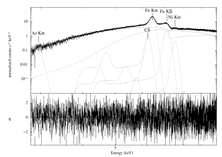
Fig. 1 XMM-Newton with ID 0555200301 (2008) orbital phase averaged spectrum of GX 301-2 in the (2.8-10.0) keV band. Top panel: data and best-fit model described by Equation (1). Bottom panel shows the residuals between the spectrum and the model. Spectral parameters can be found in Table 1 (third column).
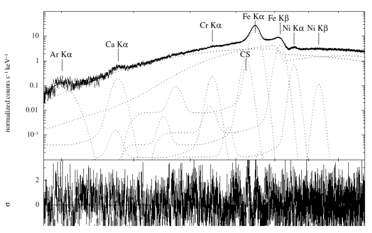
Fig. 2 XMM-Newton with ID 0555200401 (2009) orbital phase averaged spectrum of GX 301-2 in the (2.8-10.0) keV band. Top panel: data and best-fit model described by Equation (1). Bottom panel shows the residuals between the spectrum and the model. Spectral parameters can be found in Table 1 (fourth column).
The Gaussian emission lines were located at Ar Kα, Fe Kα, Fe Kβ, and Ni Kα, fluorescent line energies in the two XMM-Newton observations; mean-while, the Gaussian emission lines located at Ca Kα, Cr Kα, and Ni Kβ fluorescent line energies were only detected in the XMM-Newton observation from 2009. Moreover, the Fe Kα showed residuals when fitted with a single Gaussian and an additional Compton Shoulder was also included (Watanabe et al. 2003). The XMM-Newton observation from 2009 was also analysed by Fürst et al. (2011). They used different continuum models to fit this spectrum but they also added the same Gaussian emission lines used in this work. The XMM-Newton observation from 2008 was also studied by Roy et al. (2024). To describe this spectrum, these authors fitted a model as previously used by Fürst et al. (2011) and identified the same Kα emission lines, included the Compton Shoulder, and Fe Kβ, but Ni Kβ was not detected.
The size of emitting region on the NS surface was obtained from the bbody component by the equation:
where D is the distance to the source in kpc, F
bb is the unabsorbed flux in erg s-1 cm-2 in the energy range [2.8-10.0] keV and T
bb is the temperature in keV. Taking into account the distance to the source given by GEDR3 d(kpc) =
The intrinsic bolometric X-ray luminosity can be expressed through the unabsorbed X-ray flux of the source as:
where L
X is the X-ray luminosity, D is the distance to the source and F
no_abs is the unabsorbed flux in the [2.8-10.0] keV energy band. The observed F
no_abs for the 2008 and 2009 observations were
In Table 1, norm represents the blackbody normalisation and is related to the luminosity of the X-ray source and the distance (L
39/
An intense Fe Kα emission line (EW ≈ [0.5, 0.7] keV) with a global hydrogen column above 1024 cm-2 has been found in the analysis and it is compatible with Leahy et al. (1988, 1989), and Fürst et al. (2011) who found in this X-ray region a strong emission line Fe K visible together with a hydrogen column above 1024 cm-2.
The flux ratio between the Fe Kα and Fe Kβ allowed us to derive that the ionisation state of iron varied from Fe XII-XIII (Fe Kβ/Fe Kα =
On the other hand, the flux ratio between Ni Kαand Ni Kβ(Ni Kβ/Ni Kα = 0.23 ± 0.09) was slightly consistent with measurements in solid state metals within errors (Han & Demir 2009) in the 2009 observation.
The results mentioned above show a slightly different values between parameters from one observation to the other. In order to further study these differences, the pre-periastron flare has been analysed in the long term to find how the spectral parameters evolve with time. In addition, GX 301-2 also shows a periodic near-apastron flare with lower intensity than the pre-periastron flare and it is also included in this long term analysis. For such studies, it is also very convenient to have spectra measured at different orbital phases with uniform phase coverage. The characteristics of theMonitor of All Sky X-ray Image(MAXI), moderate energy resolution and all-sky coverage, are well suited for elaborate studies of the orbital phase resolved spectra of bright X-ray sources. The process which was used to obtain the data is explained in § 2.
Observations, data, and timing analysis are described in § 2. MAXI/GSC spectral analyses for the pre-periastron and near-apastron flares are discussed in § 3, and § 4 contains the summary of the main results.
2. TIMING ANALYSIS
The orbital phase of the pre-periastron flare has been divided into three sections to perform the spectral analysis. To define them the MAXI/GSC (2.0-20.0 keV) light curve with a time bin of 0.02 days8has been folded using the ephemeris from Koh et al. (1997), which are reported in Table 2, and a circular orbit has been assumed because we wanted to have an approximation of the results. Figure 3 shows the light curve folded over the GX 301-2 orbital period where three sections have been identified by vertical lines: I pre-flare, II flare and III post-flare. As a consequence of the low intensity level, only one section has been used to define the near-apastron flare at the [0.20-0.70] orbital phase range. For each orbit, the Modified Julian Dates (MJDs) for every orbital phase range of the pre-periastron flare have been calculated. For each section, data were accumulated over ten consecutive orbits to extract spectra with acceptable signal-to-noise ratio. As an example, Table 3 summarizes MJDs of the first ten orbits for pre-flaring, flaring and post-flaring, which were used as good time intervals (GTIs) to extract the spectra. One possible implication of the circular orbit assumption is that the MJDs would be affected by the approach of the orbit and there could be inaccuracies that could affect the conclusions obtained. However, the spectra are consistent from one set to the next one (see Figures 9-11) and this indicates that the assumption of a circular orbit is useful for the system GX 301-2 when analysing the pre-periastron flare.
TABLE 2 EPHEMERIS DATA USED FOR MAXI/GSC 'S TIMING CALCULATION
| T 0,periastron-passage (MJD) | 48802.79 ± 0.12 |
| P orb(d) | 41.498 ± 0.002 (Koh et al. 1997) |
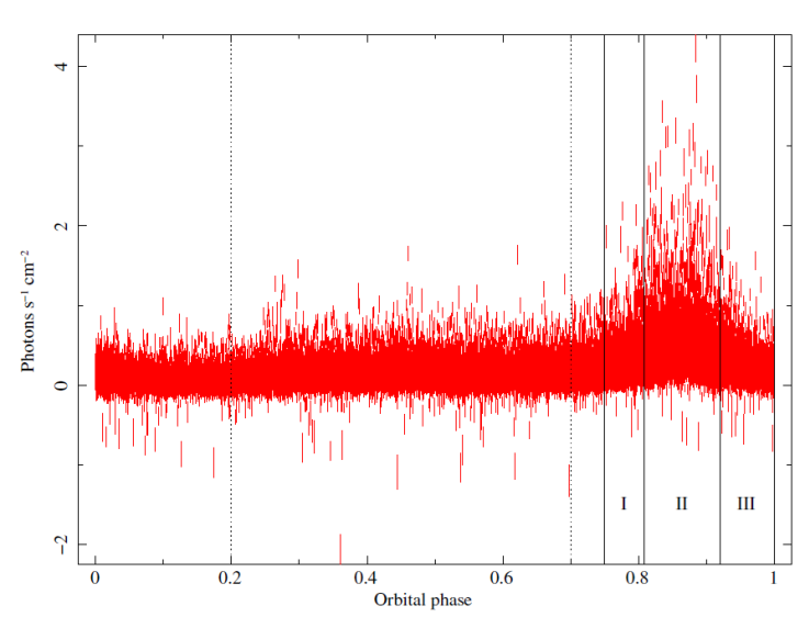
Fig. 3 Folded and background subtracted light curve in the (2.0−20.0) keV energy range. The light curve was folded over the orbital period and binned into ≈ 450 phase bins. The selection criteria for the apastron flare from MAXI data were: orbital phase range = [0.20−0.70] and (2−20) keV flux >0.5 photons cm−2 s−1. The color figure can be viewed online.
TABLE 3 FIRST TEN ORBITS: PRE-FLARE, FLARE AND POST-FLARE
| Pre-flare (≈[0.7493, 0.8090]) | Flare (≈[0.8090, 0.9205]) | Post-flare (≈[0.9205, 0.9984]) |
|---|---|---|
| MJD i -MJD f | MJD i -MJD f | MJD i -MJD f |
| 55141.582121-55144.056111 | 55144.056111-55148.686661 | 55148.686661-55151.921117 |
| 55183.080121-55185.554111 | 55185.554111-55190.184661 | 55190.184661-55193.419117 |
| 55224.578121-55227.052111 | 55227.052111-55231.682661 | 55231.682661-55234.917117 |
| 55266.076121-55268.550111 | 55268.550111-55273.180661 | 55273.180661-55276.415117 |
| 55307.574121-55310.048111 | 55310.048111-55314.678661 | 55314.678661-55317.913117 |
| 55349.072121-55351.546111 | 55351.546111-55356.176661 | 55356.176661-55359.411117 |
| 55390.570121-55393.044111 | 55393.044111-55397.674661 | 55397.674661-55400.909117 |
| 55432.068121-55434.542111 | 55434.542111-55439.172661 | 55439.172661-55442.407117 |
| 55473.566121-55476.040111 | 55476.040111-55480.670661 | 55480.670661-55483.905117 |
| 55515.064121-55517.538111 | 55517.538111-55522.168661 | 55522.168661-55525.403117 |
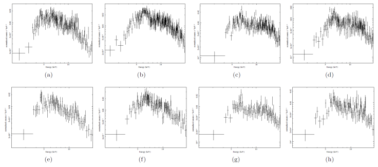
Fig. 4 MAXI/GSC spectra of GX 301-2 in the (2.0−20.0 keV) band. (a) and (e): pre-flare, third extraction. (b) and (f) pre-flare, ninth extraction. (c) and (g): post-flare, fifth extraction. (d) and (h): post-flare, eighth extraction. Spectra (a)-(d) correspond to the accumulation of ten orbits. Spectra (e)-(h) correspond to the accumulation of five orbits. Units of the x-axis: Energy (keV). Units of the y-axis: normalized counts s−1keV−1.
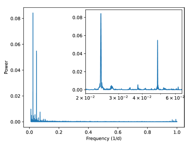
Fig. 5 Lomb-Scargle periodogram of the (4.0-10.0) keV light curve. The plot on the right top corner has been added to show only lower frequencies where the peaks lie. The color figure can be viewed online.
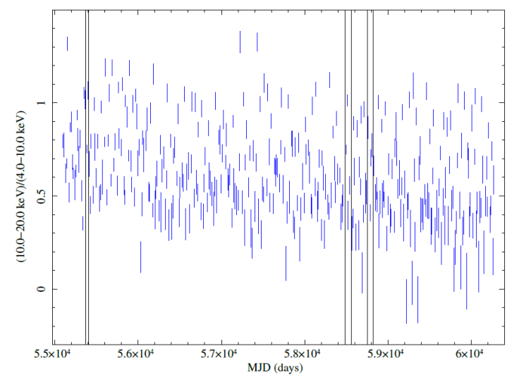
Fig. 6 Hardness ratiohard / medium=(10.0−20.0 keV)/(4.0−10.0 keV) using weighted average. The spin-up episodes are indicated by two vertical lines: (a) from MJD 55375 to 55405, (b) from MJD 58480 to 58560 and (c) from MJD 58750 to 58820. The color figure can be viewed online.
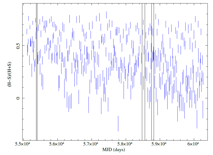
Fig. 7 Hardness curve (medium - soft)/(medium + soft) using weighted averages. The spin-up episodes are indicated by two vertical lines: (a) from MJD 55375 to 55405, (b) from MJD 58480 to 58560 and (c) from MJD 58750 to 58820. The color figure can be viewed online
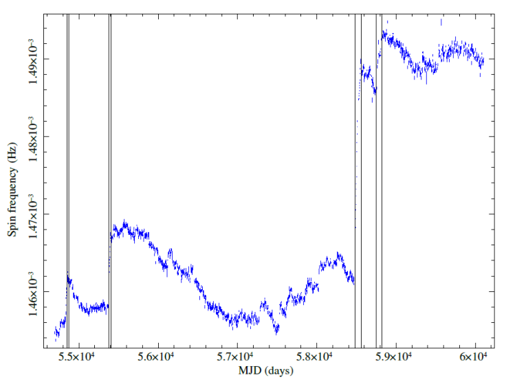
Fig. 8 Spin frequency versus the MJD for the system GX 301-2 using the data from Fermi/GBM . There are four spin-up episodes which are indicated by two vertical lines: (a) from MJD 54850 to 54870, (b) from MJD 55375 to 55405, (c) from MJD 58480 to 58560 and (d) from MJD 58750 to 58820. The color figure can be viewed online.
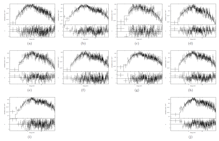
Fig. 9 MAXI/GSC spectra of GX 301-2 in the (2.0−20.0 keV) band corresponding to the pre-flare (≈ [0.7493,0.8090]), model defined by Equation (6). The same orbital phase range was accumulated in groups of ten consecutive orbits to obtain each spectrum. Units of the x-axis: Energy (keV). Units of the y-axis: normalized counts s−1keV−1.
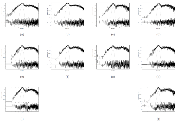
Fig. 10 MAXI/GSC spectra of GX 301-2 in the (2.0−20.0 keV) band corresponding to the flare (≈ [0.8090,0.9205]), model defined by Equation (6). The same orbital phase range was accumulated in groups of ten consecutive orbits to obtain each spectrum. Units of the x-axis: Energy (keV). Units of the y-axis: normalized counts s−1keV−1.
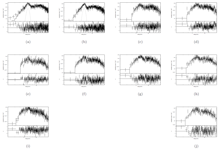
Fig. 11 MAXI/GSC spectra of GX 301-2 in the (2.0−20.0 keV) band corresponding to the post-flare (≈ [0.9205,0.9984]), model defined by Equation (6). The same orbital phase range was accumulated in groups of ten consecutive orbits to obtain each spectrum. Units of the x-axis: Energy (keV). Units of the y-axis: Normalized counts s−1keV−1.
Figure 4 shows a comparison between spectra obtained by accumulating ten orbits (top spectra) and spectra obtained by accumulating five orbits (bottom spectra).
In the context of MAXI/GSC data, the passbands often used are called "soft" (2.0−4.0) keV, "medium" (4.0−10.0) keV, and "hard" (10−20.0) keV bands. To search for pre-periastron and near-apastron changes in the X-ray emission, light curves in the (2.0−4.0) keV, (4.0−10.0) keV, (10−20.0) keV and (5.7−7.5) keV (iron complex emission lines) energy bands were extracted and analysed using Astropy, a collection of software packages which are included in Python (Astropy Collaboration et al. 2022). In each of these light curves a Lomb-Scargle periodogram (Press & Rybicki 1989) was applied and the error in the period is approximately the area where the peak is at the 90% of its value. It was apparent that the light curves were similar to each other and, in this work, only the periodogram of the light curve (4−10 keV) is shown (see Figure 5). As can be seen from Figure 5, the highest peak (power ≈ 0.084) is at (41.4 ± 0.5) days which corresponds to the rotational period of the binary system determined by Koh et al. (1997). The second peak (power ≈ 0.055) in the power density spectrum at ≈ 20.7 days is potentially a harmonic of the orbital period.
The hardness ratio is a specially useful tool to quantify and characterise the source spectrum. Therefore, simple hardness ratio (hard/medium) and fractional difference hardness ratio (medium−soft)/(medium+soft) have been calculated using the weighted average over 150 bins and plotted in Figures 6 and 7, respectively. The weighting factor here for computing the average HR is the error weighted average, where the errors have been calculated with the general method of using formulas for propagating errors. Both graphs show that the ratios continue to oscillate around the average, with no clear trend.
Figure 8 shows the pulse frequency history of GX 301-2 observed with Fermi/GBM Accreting Pulsars Program9(Malacaria et al. 2020). Every two vertical lines on this plot represent a spin-up episode in the history of observations of the source, which have been associated with the formation of a transient accretion disc (Koh et al. 1997; Nabizadeh et al. 2019). Two of these irregular spin-up episodes can be related to the apastron passages (see § 3.2).
3. SPECTRAL ANALYSIS
3.1. Pre-periastron Flare Spectra
The spectra were obtained using the MAXI/GSC on-demand process10; all of them were analysed and modelled with the XSPEC (Arnaud 1996) package and the energy range used for spectral fitting was (2.0-20.0) keV. Both phenomenological and physical models commonly applied to accreting X-ray pulsars have been tested. Models with power law components have been developed to HMXBs, such as Cen X-3 (Ebisawa et al. 1996) and GX 301-2 (Fürst et al. 2011; Ji et al. 2021). First of all, traditional models like power law with a high energy cut-off or with a Fermi-Dirac cut-off were explored. Although these models reasonably well reproduce the observed flare spectra between (2.0−20.0 keV) (
Although both models described above fitted the averaged spectra between (2.0−20.0 keV) with a similar statistical confidence (Equation 4,
During flare episodes the surface temperature of the neutron star can reach several million degrees and, therefore, it will emit blackbody radiation with photons in the X-ray range. The blackbody component has been used to describe the soft energy band spectra of HMXBs like Cen X-3 using data from XMM-Newton (Sanjurjo-Ferrín et al. 2021) and MAXI/GSC (Torregrosa et al. 2022). The overall MAXI/GSC spectra of the source was modelled with an absorbedbbodycomponent. The spectral shape showed evidence for an Fe K-shell absorption edge at ≈ 7.1 keV (Saraswat et al. 2006; Endo et al. 2002; Ji et al. 2021); therefore, an edge component fixed at this energy was added. The following model was applied to describe all observational data:
where the Gaussian line was also included to account for the iron fluorescent emission line at ≈ 6.4 keV, if present. The model gave a good statistical description (pre-flare,
Some spectra showed a low-energy excess below ≈4.0 keV as can be seen in Figure 9, images (b), (c), (g), (i) and (j); Figure 10, image (g); and Figure 11, images (g), (h) and (j). This soft excess could be produced by a transitory structure in the line of sight because it was not a permanent effect in all X-ray spectra. Therefore, a possible explanation may be the presence of a transitory disc which enhances the accretion of matter. X-ray pulsars such as GX 301-2 tend to be spinning up because the accreted material from the optical star has an angular momentum which is eventually transferred to the compact object. The higher the X-ray luminosity, the more material is accreted by the pulsar, and therefore the faster it will spin. The strongest spin-up event of GX 301-2 so far (between December 2018 and March 2019) pointed to an accretion due to both direct accretion from the stellar wind and a temporary accretion disc (Nabizadeh et al. 2019). This scenario was also supported by the observations taken with theInsight-Hard X-ray Modulation Telescopeduring the initial part of this spin-up episode (Liu et al. 2021). On the other hand, the low-energy excess could also be explained by scattering in the gas stream around the neutron star and in the stellar wind of the B-type companion star (Saraswat et al. 1996).
Figures 12 to 19 show the evolution of the best-fit model parameters during the pre-periastron and apastron passages. In Figures 13-19 filled black squares represent the pre-flare parameter values, filled red triangles the flare parameter values, and open blue circles the post-flare parameter values.
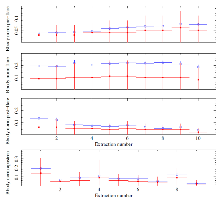
Fig. 12 Evolution of the bbody norm for the pre-periastron flare and apastron outbursts versus the extraction number (MAXI/GSC data, model defined by Equation 6). Top panel: pre-flare. Second panel: flare. Third panel: post- flare. Bottom panel: apastron out-bursts. Filled red squares: bbody norm calculated by using L
39/
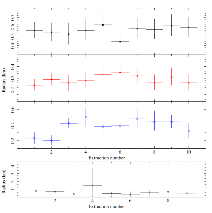
Fig. 13 Evolution of the radius of the emission zone for the pre-periastron flare and apastron outbursts versus the extraction number (MAXI/GSC data, model defined by Equation 6). Filled black squares: pre-flare. Filled red triangles: flare. Open blue circles: post-flare. Filled dark grey stars: apastron outbursts. The color figure can be viewed online.
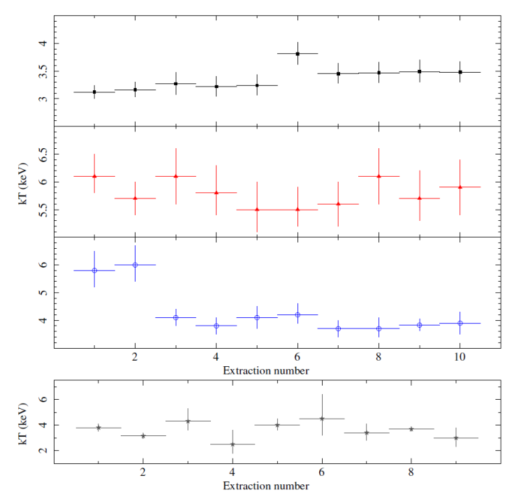
Fig. 14 Evolution of the bbody temperature for the pre-periastron flare and apastron outbursts versus the extraction number (MAXI/GSC data, model defined by Equation 6). Filled black squares: pre-flare. Filled red triangles: flare. Open blue circles: post-flare. Filled dark grey stars: apastron outbursts. The color figure can be viewed online.
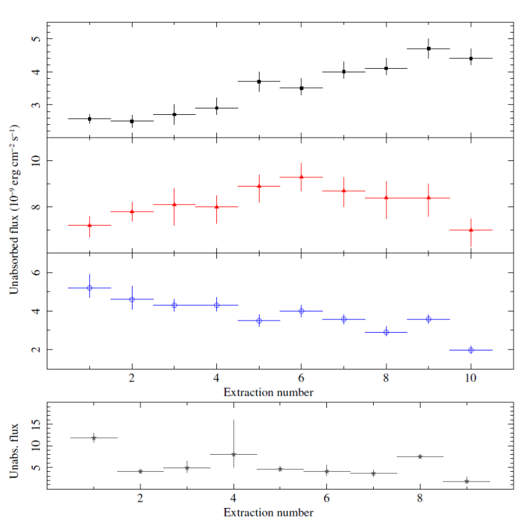
Fig. 15 Evolution of the unabsorbed flux for the pre-periastron flare and apastron outbursts (in units of 10-9 erg cm-2 s-1) versus the extraction number (MAXI/GSC data, model defined by Equation 6). Filled black squares: pre-flare. Filled red triangles: flare. Open blue circles: post-flare. Filled dark grey stars: apastron outbursts. The color figure can be viewed online.
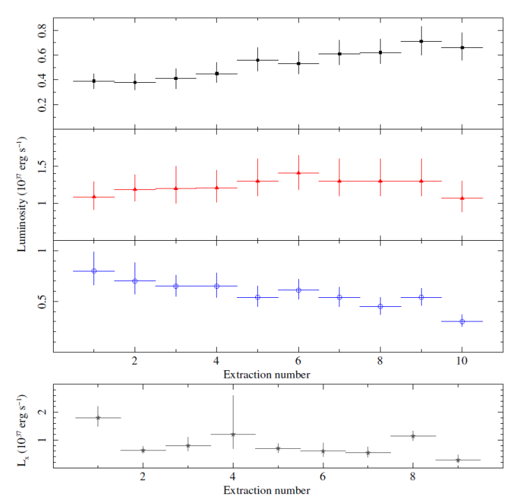
Fig. 16 Evolution of the luminosity for the pre-periastron flare and apastron outbursts versus the extraction number (MAXI/GSC data, model defined by Equation 6). Filled black squares: pre-flare. Filled red triangles: flare. Open blue circles: post-flare. Filled dark grey stars: apastron outbursts. The color figure can be viewed online.
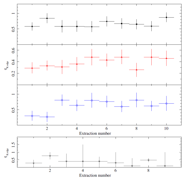
Fig. 17 Evolution of the optical depth of the edge for the pre-periastron flare and apastron outbursts versus the extraction number (MAXI/GSC data, model defined by Equation 6). Filled black squares: pre-flare. Filled red triangles: flare. Open blue circles: post-flare. Filled dark grey stars: apastron outbursts. The color figure can be viewed online.
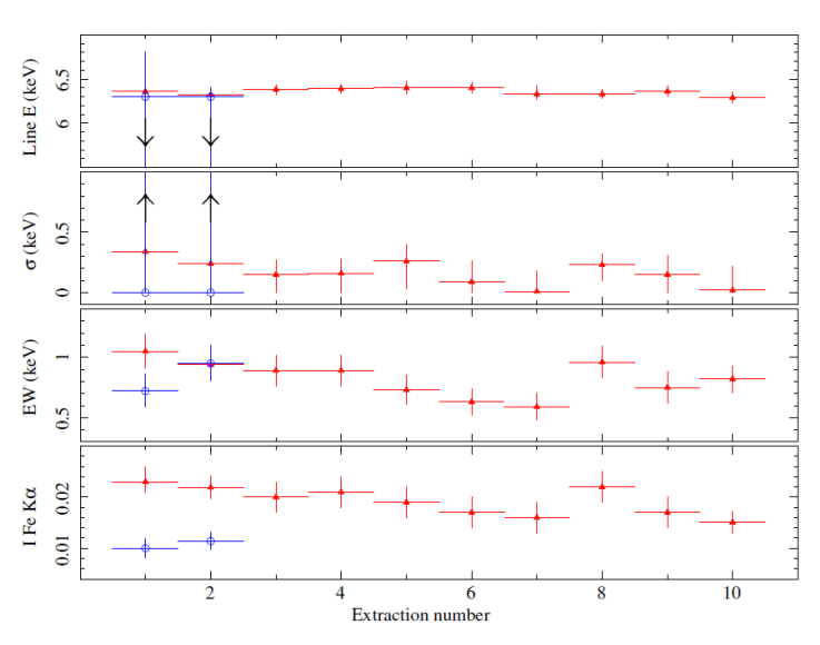
Fig. 18 The parameters of the Fe Kα emission line versus the extraction number (MAXI/GSC data, model defined by Equation 6). Top panel: line energy. Second panel: line width. Third panel: equivalent width. Bottom panel: intensity. The unit of the line flux I is photons s-1 cm-2. Filled red triangles: flare. Open blue circles: post- flare. The color figure can be viewed on-line.
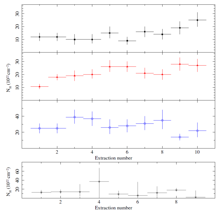
Fig. 19 Evolution of the column density for the pre-periastron, flare, and apastron outbursts versus the extraction number (MAXI/GSC data, model defined by Equation 6). Filled black squares: pre-flare. Filled red triangles: flare. Open blue circles: post-flare. Filled dark grey stars: apastron outbursts. The color figure can be viewed online.
Taking the uncertainties into account, the results for thebbody normalisation(Figure 12) obtained with XSPEC (open blue circles) are consistent with the values obtained usingL
39/
The radius of the emission zone (Figure 13) is of the order of 1 km, which is consistent with a hot spot on the NS surface and with the results of XMM-Newton data. The temperature of the blackbody (kTin keV, Figure 14) has a constant value between (3.0−3.5) keV in the pre-flare spectra, but it is enhanced in the sixth extraction, which is reflected in a drop of the emission radius (Figure 13). In the flare spectra, it is enhanced in the (5.5-6.5) keV range indicating an increase in the accretion rate which is reflected in a higher X-ray luminosity compared to pre-and post-flare. In the post-flare the temperature is approximately constant, (3.8-4.1) keV, between the third and the tenth extraction, but there is a large increase in the first and second extractions with a value ≈ 6.0 keV which is reflected in a clear decrease of the emission zone between ≈ (0.2-0.3) km.
In the flare the unabsorbed flux (Figure 15) has no significant evolution in the fitting energy range (2.0-20.0) keV, showing that the accretion rate is quite stable. The unabsorbed fluxes show opposite trends between the pre-flare (the flux increases) and the post- flare (the flux decreases) showing that the accretion rate has a different behaviour along the pre-periastron passage. A possible explanation for this would be that the absorbing matter is located in the line of sight between the observer and the neutron star in the post- flare (N H ≳ 2 1023 cm-2) and away from the line of sight in the pre-flare (N H < 2 1023 cm-2). Thus, it is confirmed that the distribution of circumstellar matter around the compact object is rather inhomogeneous during the pre-periastron passage (Saraswat et al. 1996; Islam & Paul 2014).
The X-ray luminosity (Figure 16) is consistent with a constant value (L X ≈1.3 × 1037 erg s-1) in the flare spectra (which agrees with the observations ID 0555200301 and ID 0555200401 from XMM-Newton) and is greater than in the pre-flare (L X = [4 - 7] 1036 erg s-1) and in the post-flare (L X = [3 - 8] 1036 erg s-1) spectra. This scenario, in which the wind mass-loss rate is insufficient to power the source entirely, indicates that an additional mechanism is needed to give the neutron star the fuel it needs. Wind-fed HMXBs are powered by accretion of the radiatively driven wind of the luminous component on the compact object with typical X-ray luminosities ≈1036 erg s-1 (see Martínez-Nuñez et al. 2017; Kretschmar et al. 2019, for instance), i.e. one order of magnitude smaller than observed in the flare event. A possible mechanism for enhancing the X-ray emission is thought to be the presence of a gas stream trailing the neutron star (Saraswat et al. 1996; Islam & Paul 2014). Another cause could be that an accretion disc has formed around the neutron star (Nabizadeh et al. 2019; Liu et al. 2021) or a combination of both possibilities (Saraswat et al. 1996). Spin-up episodes are usually characterised by an increase in X-ray luminosity, associated with an enhancement of the accreted matter as a consequence of the formation of a temporary accretion disc around the neutron star (Nabizadeh et al. 2019; Manikantan et al. 2023).
This source is seen through a column density in the range N H = [10-40] 1022 cm-2, and all X-rays below [2-3] keV are absorbed. At these column densities a feature due to the K edge of Fe at 7.1 keV should be present. Figure 17 shows the optical depth of the iron edge (τ Kedge) best-fit parameter that lies in the range [0.3 - 0.8]. This represents an ionisation state of nearly neutral iron Fe i-v (if values reported by Saraswat et al. 1996; Endo et al. 2002; Ji et al. 2021, are taken into account).
The long-term averaged spectra in the flare section present a fluorescent iron emission line energy consistent with the Fe Kα line and a constant value of ≈ (6.35±0.08) keV, as can be seen in Figure 18, top panel, which implies an ionisation state of iron up to Fe XVII. It was only detected in the first two spectra in the post-flare section and it was totally absent in the pre- flare section. However, Islam & Paul (2014) performed an orbital phase-resolved spectral analysis of GX 301-2 and they reported that the iron emission line was detected in all the orbital phases. The fitted values of the line width, the equivalent width and the intensity of the Fe Kα emission line are plotted in Figure 18: second, third and bottom panels, respectively.
If the emission line luminosity is produced by a thin spherical shell of matter, i.e. a shell of gas surrounding a point source of continuum radiation with uniform ionisation, composition and density, the line equivalent width should be proportional to the column density (Kallman et al. 2004; Torrejón et al. 2010) EW line(keV) ≃ 0.3 N H (1024 cm-2). The absorbing component varies in the range ≈ [10-30] × 1022 cm-2 (see second panel from the top of Figure 19), which implies an equivalent width of Fe Kα in the range EW line ≈ [30-90] eV. On the other hand, for an isotropic surrounding cosmic fluorescing plasma, Inoue (1985) obtained a relationship between the expected equivalent width of the iron Kα line and the hydrogen column density as EW expected(eV) = 100 N H (1023 cm-2) which is valid for N H < 1024 cm-2 and a photon index of the power-law spectrum of 1.1 (see also Endo et al. 2002, for example). They also concluded that GX 301-2 corresponds to this case and, therefore, EW line ≈ [100-300] eV. However, MAXI/GSC observations gave equivalent widths of the iron emission line in the range EWline ≈ [600-1100] eV, which implies large deviations from the linear correlation. The largest value of the equivalent width was obtained with the smallest column density. The fact that the Fe Kα is not a single line but a superposition of different Kα lines of differently strongly ionised iron together with the Compton shoulder at ≈6.24 keV and the wind speed could explain the large equivalent widths found in this study (Watanabe et al. 2003; Fürst et al. 2011; Ji et al. 2021). Taking the uncertainties into account, the best-fit parameters in the pre-periastron orbital phase are consistent with previous studies (Islam & Paul 2014; Manikantan et al. 2023). As a consequence, during the pre-periastron passage the fluorescent iron emission line is not emitted from a spherically symmetric distribution of matter surrounding the neutron star. Although this study has focused on flare episodes, a very small part of the orbit, these results are consistent with those obtained by Islam & Paul (2014).
Figure 20 shows the equivalent width of the Fe Kα against the absorption column density during the pre-periastron passage compared with the theoretical predictions for an isotropically distributed gas and for a spherical shell of gas surrounding the source. In fact, it seems that there is a moderate anti-correlation between them during the pre-periastron passage and a Pearson correlation coefficient r = -0.63 was found. This result is in contrast to other studies, such as Makino et al. (1985), Endo et al. (2002), Fürst et al. (2011), Ji et al. (2021), where they found a linear correlation between these two parameters which suggests that the accretion material near the neutron star is spherically distributed. Nevertheless, Ji et al. (2021) also found deviations from this linear correlation when the column density was higher than 1.7 × 1024 cm-2. They pointed out that this could be due to the formation of an accretion disc.
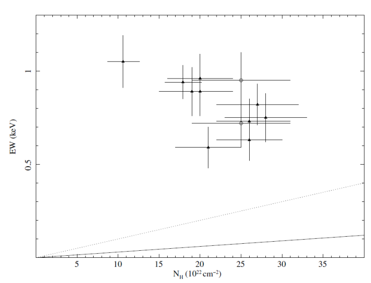
Fig. 20 Variability of the equivalent width as a function of the column density (also known as the curve of growth). Filled black triangles: flare. Open black circles: post-flare. The dotted line represents the relation for an isotropic surrounding cosmic fluorescing plasma, EW expected(eV) = 100 N H (1023 cm-2) (Inoue 1985). The solid line shows the relation for the luminosity produced by a thin spherical shell of matter EW line(keV) ≃ 0.3 N H (1024 cm-2) (Kallman et al. 2004; Torrejón et al. 2010).
In Figure 21 the intensity of the Fe Kα emission line is shown versus the unabsorbed flux of the source in the [2-20] keV energy band (left plot) and the optical depth of the iron K-edge absorption versus the equivalent width of the iron Kα line (right plot). A moderate linear correlation (Pearson correlation coefficient r = 0.63) can be seen, which should be consistent with the expected line intensities for the hydrogen column densities derived from the model described by Equation 6 (see fig.6b in Haberl 1991b, where the incident spectrum was assumed to be a power-law with photon index Γ = 0.55). In contrast, from the plot τ edge versus EW, an anticorrelation relationship (Pearson correlation coefficient r = -0.75) seems to be present between these parameters during the pre-periastron passage. The solid line represents the linear fit found by Ji et al. (2021) where they suggested that the reprocessed material reached an optical depth of unity for EW ≈ 400 eV (see also Torrejón et al. 2010, where they also found a linear correlation).
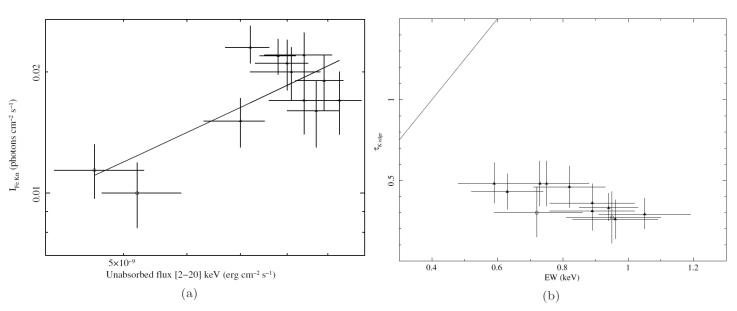
Fig. 21 Left panel: Log-log plot of the Fe Kα intensity as a function of the unabsorbed flux in the (2-20) keV energy band. The solid line represents a linear fit. Right panel: Plot of the optical depth of the iron K-edge absorption as a function of the equivalent width of the iron Kα line (in keV). The solid line is the linear fit found by Ji et al. (2021). An apparent anti-correlation can be seen during the pre-periastron passage. The larger the EW of the Fe Kα, the smaller the optical depth of the iron K-edge absorption. Filled black triangles: flare. Open black circles: post-flare.
3.2. Apastron Flare Spectra
The folded light curve of GX 301-2 shows two flare-like features at binary orbital phases ≈ 0.26, i.e. before apastron passage (Haberl 1991b; Saraswat et al. 1996), and at ≈ 0.45 near-apastron passage (as can be seen in Figure 3, see also Pravdo et al. 1995; Pravdo & Ghosh 2001, for instance). In general, periodic near-apastron outbursts show lower intensity than the pre-periastron flare, although X-ray emission can sometimes be as low as ≈ 1036 erg s-1, i.e. it cannot be distinguished from the baseline X-ray intensity along the orbit. Thus, the criterion to identify an apastron outburst was that the unabsorbed X-ray flux was greater than ≈ 2 × 10⁻⁹ erg s-1 cm-2. The orbital phase of the apastron outbursts was also obtained with the parameters reported by Koh et al. (1997). Then, the Good Time Intervals (GTIs) were derived and the corresponding MJDs are listed in the caption of Figure 22. Finally, the spectra were extracted following the process explained in § 3.1.
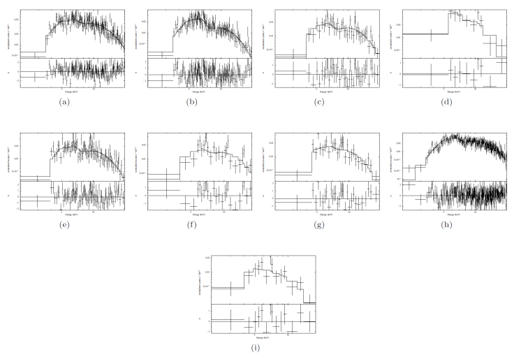
Fig. 22 MAXI/GSC spectra of GX 301-2 in the [2.0-20.0] keV band corresponding to the apastron flare. MJDs from left to right for each spectrum: (a) [55376.5-55380.5], (b) [55710.0-55713.0], (c) [55870.0.0-55873.0], (d) [56163.5-56164.5], (e) [57285.0-57288.0], (f) [57454.0-57457.0], (g) [58029.5-58041.5], (h) [58480.5-58495.5] and (i) [59119.0-59122.0]. Units of the x-axis: Energy (keV). Units of the y-axis: Normalized counts s-1 keV-1.
In this analysis, all apastron spectra were fitted with the same model used for the pre-periastron flare spectra. The range of the
The unabsorbed fluxes and the derived radii of the blackbody emission region are shown in Figures 15 and 13, respectively. The results for the radii are consistent with a hot spot on the NS surface (Sanjurjo-Ferrín et al. 2021; Torregrosa et al. 2022) (see Table 4, Column 3).
TABLE 4 SELECTED FIT PARAMETERS FROM APASTRON FLARE SPECTRA
|
|
|
|
|
|
|
|---|---|---|---|---|---|
| 1 | 55376.5-55380.5 [0.41-0.51] |
|
|
|
|
| 2 | 55710.0-55713.0 [0.45-0.52] |
|
|
|
|
| 3 | 55870.0-55873.0 [0.30-0.37] |
|
|
|
|
| 4 | 56163.5-56164.5 [0.38-0.40] |
|
|
|
|
| 5 | 57285.0-55288.0 [0.40-0.47] |
|
|
|
|
| 6 | 57454.0-57457.0 [0.47-0.55] |
|
|
|
|
| 7 | 58029.5-58041.5 [0.34-0.63] | 0.6 |
|
|
|
| 8 | 58480.5-58495.5 [0.21-0.57] | 0.68 |
|
|
|
| 9 | 59119.0-59122.0 [0.60-0.67] |
|
|
|
|
Using the definition of the bbody normalisation K
bb = L
39/
The first apastron outburst spectrum observed by MAXI/GSC is shown in Figure 22 (a) whose X-ray luminosity, see Table 4, Column 6, L
X(a)
≈ 2 × 1037 was unusually brighter than that of pre-periastron flare (see Figure 16 and compare second and bottom panels). This flare was also detected by Fermi/GBM and could be associated with a rapid spin-up episode of GX 301-2 (Finger et al. 2010). According to the long-term light curve obtained with Fermi/GBM, rapid spin-up began on June 23, 2010 (MJD 55 370.84) and finished on July 22, 2010 (MJD 55 399.07), as can be seen in Figure 8. Pulse timing measurements for the interval June 23.8-July 22.1 showed a spin-up frequency rate of
Another rapid spin-up episode seen with Fermi/GBM from MJD 54 830.9617 to MJD 54 855.1007 showed a spin-up frequency rate of
The rest of the apastron flares shown in Figures 22 (b), (c), (e), (f), (g) and (i) had an X-ray emission slightly lower than pre-periastron flares which were not associated with any significant changes in the spin period of the neutron star. From MJD 55 708.9521 to MJD 55 714.8995, the spin-up rate was
As far as it is known from the rapid spin-episodes in GX 301-2, during the apastron passage the source becomes as bright as a pre-periastron flare, as a consequence of the formation of a transitory accretion disc. Thus, the mass transfer from the companion star to the neutron star is a rather irregular process during this orbital phase (see X-ray luminosities in Table 4). The strongest events show that the material is accreted from the stellar wind, possibly from a gas stream (Leahy & Kostka 2008) and probably through a temporary accretion disc (Koh et al. 1997; Nabizadeh et al. 2019; Abarr et al. 2020; Liu et al. 2021; Manikantan et al. 2023). However, the fourth apastron flare [see extraction number 4 in Table 4 and Figure 22 (d)] did not show a spin-up of the neutron star and no transitory disc was formed. Therefore, the material should be accreted by the stellar wind and possibly from a gas stream.
It should be noted that the uorescence iron emission line at ≈6.4 keV has not been detected in any spectrum of the apastron flare. Sensitive X-ray observatories such as ASCA (Endo et al. 2002), XMM-Newton (Giménez-García et al. 2015), and Chandra (Torrejón et al. 2010) detected and resolved the iron line complex in GX 301-2. In contrast, MAXI/GSC does not have enough sensitivity to distinguish between a weak, broad iron K emission line and a bright X-ray continuum (Rodes-Roca et al. 2015; Torregrosa et al. 2022). Nevertheless, other long-term orbital phase resolved spectroscopy studies reported the presence of the Fe Kα line in all orbital phases (Islam & Paul 2014; Manikantan et al. 2023).
4. SUMMARY AND CONCLUSIONS
The main goal of the current study was to determine the long-term variation of GX 301-2 in the pre-periastron and apastron flares. The Good Time-Intervals corresponding to these orbital phases were generated using the orbital ephemeris from Koh et al. (1997).
The main results can be summarise as follows: - From the analysis of the MAXI/GSC (4.0-10.0) keV light curve, we have estimated the orbital period of the binary system, P orb = 41.4±0.5 days, being in agreement with the best value derived by Koh et al. (1997).
- Two variations of the model tbnew × po + tbnew × po + GL have been applied to find if there was elliptical polarisation due to synchrotron radiation. This model was not able to describe all MAXI/GSC data properly.
- The size of the emitting region on the neutron star surface in the pre-periastron and apastron flares obtained using the bbody normalisation (see Figure 13 and Table 4) was compatible with a hot spot. The temperature of the blackbody is in the range [5.1-6.7] keV during the pre-periastronv and two post-flare, but lower than 5.0 keV in the rest of the spectra. It was not clear if there is a connection between the high temperature of the blackbody and the detection of the iron K line.
- The X-ray luminosity during the pre-periastron flare was compatible with a constant value (L X ≈ 1.3 × 1037 erg s-1) indicating an accretion rate quite regular from the stellar wind and a gas stream trailing the neutron star (Leahy & Kostka 2008). This mass transfer model would also explain the X-ray luminosities obtained in the pre-flare (L X = [4-7] × 1036 erg s-1), in the post- flare (L X = [3-8] × 1036 erg s-1) and in most of the apastron flares (L X = [3-8] × 1036 erg s-1). However, two of the strongest apastron flares had an X-ray luminosity comparable to the pre-periastron are during rare spin-up events. It is believed that a certain amount of angular momentum should be transported through the formation of an accretion disc at this orbital phase (Nabizadeh et al. 2019; Abarr et al. 2020; Manikantan et al. 2023). At least one of the largest apastron flares (extraction number 4 in Table 4) was not related to a spin-up episode and, therefore, it is quite likely that a transient accretion disc did not form. Consequently, it remains unknown why only some apastron flares spin up the X-ray source and on what this depends.
- The curve of growth showed a moderate anti-correlation between the equivalent width of Fe Kα and the column density, and clear deviations from spherically distributed absorbing matter (Kallman et al. 2004; Islam & Paul 2014; Giménez-García et al. 2015; Ji et al. 2021) in the pre-periastron flare. On the other hand, a moderate correlation between the unabsorbed X-ray flux and the intensity of Fe Kα was found, which could be consistent with the expected values corresponding to the hydrogen column densities in the pre-periastron flare (see figure 6b in Haberl 1991b).
- The optical depth of the K-edge absorption was moderately anti-correlated to the equivalent width of Fe Kα, and clearly deviated from the linear correlation reported by Ji et al. (2021) (see also the result obtained by Torrejón et al. 2010).

