Articles
Discovery of 28 Open Clusters with Gaia DR3

-
Publication dates-
December 05, 2025
Jan-Jun , 2025
- Article in PDF
- Article in XML
- Automatic translation
- Send this article by e-mail
- Share this article +
Abstract
In this work we searched for open clusters in the fields of star-forming regions in the Galaxy using the HDBSCAN applied to the astrometric data from the Gaia DR3 catalog. We identified 28 new open clusters, of which the real existence is supported by the membership probability determined from astrometric data and by the presence of cluster sequences in their color-magnitude diagrams, which allows for a reliable isochrone fit. Of the open clusters identified, 3 are younger than 50 Myr, 19 are of intermediate age, and 6 are old clusters. The clusters have apparent radii ranging from 3 to 20 arcmin. For all clusters, we estimate mean proper motion, mean parallax, and fundamental parameters considering the member stars for each cluster. One of the discovered clusters has a distance of 10 kpc and a log(age) ≈ 10.1, making it one of the most distant and oldest cataloged open clusters.
Key Words::
open clusters and associations: general
1. INTRODUCTION
Open clusters (OCs) are key objects used to study the structure and dynamics of the Galaxy since their kinematics, distances, and ages can be determined with good precision from the properties of their member stars.
Before the Gaia era, the most widely used catalogs of OCs and their fundamental parameters were the New Catalog of Open Clusters and Candidates (Dias et al. 2002) and the Milky Way Star Clusters (Kharchenko et al. 2003), both of which contain about 3 thousand objects.
-
Dias et al. 2002A&A, 2002
-
Kharchenko et al. 2003ARep, 2003
This scenario changed with the new generation of high precision all-sky astrometric Gaia catalogs, which provided data to limiting magnitude about 21, offering an important opportunity to determine the parameters and members of the known open clusters as well as to discover new ones.
Recently, many works have used clustering algorithms, supervised or not, to search for new open clusters and to identify their member stars: He et al. (2022) used the pyUPMASK algorithm (Pera et al. 2021) with the K-means clustering method; Castro-Ginard et al. (2020), Castro-Ginard et al. (2019) and Hao et al. (2022) used DBSCAN (Ester et al. 1996); Cantat-Gaudin & Anders (2020) used the UPMASK procedure (Krone-Martins & Moitinho 2014); Liu Pang (2019) used the Friend of Friends method; Sim et al. (2019) used Gaussian mixture model and mean-shift algorithms; Jaehnig et al. (2021) used extreme deconvolution Gaussian mixture models; and recently Kounkel & Covey (2019), Kounkel et al. (2020), Hunt & Reffert (2021) and Hunt & Reffert (2023) used HDBSCAN to search for open clusters.
-
He et al. (2022)ApJS, 2022
-
Pera et al. 2021A&A, 2021
-
Castro-Ginard et al. (2020)A&A, 2020
-
Castro-Ginard et al. (2019)A&A, 2019
-
Hao et al. (2022)A&A, 2022
-
Ester et al. 1996Proc. of 2nd International Conference on Knowledge Discovery and Data Mining (KDD-96), 1996
-
Cantat-Gaudin & Anders (2020)A&A, 2020
-
Krone-Martins & Moitinho 2014A&A, 2014
-
Liu Pang (2019)ApJS, 2019
-
Sim et al. (2019)JKS, 2019
-
Jaehnig et al. (2021)ApJ, 2021
-
Kounkel & Covey (2019)AJ, 2019
-
Kounkel et al. (2020)AJ, 2020
-
Hunt & Reffert (2021)A&A, 2021
-
Hunt & Reffert (2023)A&A, 2023
As a direct consequence of the publication of the Gaia catalogs and the application of advanced machine learning techniques, currently about 8000 open clusters are known and cataloged (Hunt & Reffert 2023), representing an almost fourfold increase in the number of clusters originally cataloged in our database (Dias et al. 2002). However, according to Hunt & Reffert (2024), the Milky Way contains a total of one hundred thousand open clusters, of which only about 4% have been discovered.
-
Hunt & Reffert 2023A&A, 2023
-
Dias et al. 2002A&A, 2002
-
Hunt & Reffert (2024)Improving the open cluster census III. Using cluster masses, radii, and dynamics to create a cleaned open cluster catalogue, 2024
In this context, we have dedicated special attention to the task of a systematic search for previously unknown open clusters, and in this work we present the first results of a search for these objects in the fields from the catalog of star-forming regions in the Galaxy published by Avedisova (2002).
-
Avedisova (2002)ARep, 2002
In the next section, we describe the procedures adopted in the search for clusters and the tools used in their analysis. § 3 is dedicated to the presentation of the isochrone fitting procedure to determine distance and age, which indicates that the clusters are real. In § 4 we discuss the results. Finally, in § 5 we give some concluding remarks.
2. CLUSTER SEARCH AND ANALYSIS STRATEGY
In this work we searched for open clusters in the fields of one degree squared centered on the star formation regions provided in the catalog published by Avedisova (2002). Basically we applied the HDBSCAN (Hierarchical Density-Based Spatial Clustering of Applications with Noise) clustering algorithm (Campello et al. 2015, 2013) in two steps, firstly to find all the clusters in each field, and subsequently to estimate the membership for stars in open clusters. These procedures are described below.
-
Avedisova (2002)ARep, 2002
-
Campello et al. 2015ACM Transactions on Knowledge Discovery from Data (TKDD), 2015
-
2013Density-Based Clustering Based on Hierarchical Density Estimates, 2013
2.1. Searching for Clusters
The HDBSCAN algorithm is an interesting method for searching for open clusters since it can identify clusters with different shapes and density, being efficient and relatively fast in dealing with large volumes of data, as is the case with the Gaia catalog. Some advantages of the method that make it more robust are its ability to deal with multidimensional data and the fact that it does not require the number of clusters to be initially defined.
As an evolution of the DBSCAN algorithm (Ester et al. 1996) it only requires the definition of the parameters min_cluster_size (minimal size to consider a cluster) and min_samples (primarily controls how tolerant the algorithm is towards noise). The other parameter is the cluster_selection_method used to select the clusters from the cluster tree hierarchy. While EOM (Excess of Mass) method produces clusters with large areas, the leaf method produces small homogeneous clusters.
-
Ester et al. 1996Proc. of 2nd International Conference on Knowledge Discovery and Data Mining (KDD-96), 1996
However, the obtained results from HDBSCAN depend on the data as well as the setup defined to use the algorithm. We refer the reader to the work of Hunt & Reffert (2021) to search for open clusters for a complete description and use of the HDBSCAN algorithm, including tests with different setups and comparisons of their performance with other methods.
-
Hunt & Reffert (2021)A&A, 2021
In this work we applied the Python code of the HDBSCAN2 in an unsupervised fashion, to find all the clusters in each field, considering a five-dimensional astrometric space (position in the tangent plane, parallax, and proper motions). We followed the results of Hunt & Reffert (2021) and set the parameters min_cluster_size = 15, min_samples = 80 and method = leaf. We also scaled the data set to have a median of zero and a unit inter-quartile range using a RobustScaler object from scikit-learn (Pedregosa et al. 2011). Clusters with fewer than 15 stars were disregarded in our analyses.
-
Hunt & Reffert (2021)A&A, 2021
-
Pedregosa et al. 2011Journal of Machine Learning Research, 2011
In Figure 1 we present the typical results for this procedure using the field 213.07-2.23 as an example, where four groups were found. In the plot, the member stars of each cluster as originally defined by the algorithm are presented in different colors. In this field three known clusters were found that were colored red for CWNU_1774, green for UBC_212 and cyan for FSR_1077, and one unknown detected open cluster (Dias_21), presented in blue color.
Thumbnail
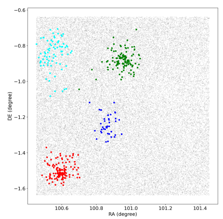
Fig. 1
The sky map with field of one degree centered in the field 213.07-2.23 is presented. In the plot, stars members as originally defined by the HDBSCAN algorithm, of each cluster are shown in different colors. In red for CWNU_1774, green for UBC_212 and cyan for FSR_1077. The stars in blue are members of Dias_21, new detected open cluster. The color figure can be viewed online.
The sky map with field of one degree centered in the field 213.07-2.23 is presented. In the plot, stars members as originally defined by the HDBSCAN algorithm, of each cluster are shown in different colors. In red for CWNU_1774, green for UBC_212 and cyan for FSR_1077. The stars in blue are members of Dias_21, new detected open cluster. The color figure can be viewed online.
The list of detected clusters was cross-referenced with the most recent publications on new open clusters, as well as with the catalog published by Hunt & Reffert (2023). In this process, we considered as new open cluster candidates those in which the central coordinates differed by more than 5 arcmin, mean proper motion differed by more than 2σ, and mean parallax differed by more than 5σ (to consider large errors for more distant stars) of the known open clusters cataloged.
-
Hunt & Reffert (2023)A&A, 2023
Subsequently, we used the Aladin Sky Atlas (Bonnarel et al. 2000) which provides tools that help ensure that the member stars of these new candidates did not correspond to members of known clusters, since these new open clusters can be in the same field (or close) to known open clusters, as is the case of Dias_21 in the field of the three known clusters as shown in Figure 1.
-
Bonnarel et al. 2000A&AS, 2000
The candidates listed as uncataloged open clusters had their color-magnitude diagram (CMD) checked by a visual inspection, and only those with a clear typical cluster sequence in the CMD were kept. We selected 28 unknown open cluster candidates and, for each of these cases, performed a more detailed analysis to determine the member stars, to apply the isochrone fit, and to determine their distances and ages.
2.2. Memberships
A recent addition to the HDBSCAN library is the introduction of soft clustering3, which capitalizes on the smoothed density function provided by the condensed tree over the data points. In this approach, cluster labels are not directly assigned to points; rather, each point receives a probability assignment. However, the probability calculations still rely on specified parameters, such as min cluster size and min samples. Here we adopt this probability estimation for the membership of the stars.
Since the results provided by the HDBSCAN algorithm depend on the parameters, we applied the code in a different way to ensure an unbiased membership determination for stars in open clusters. In this approach we use a Monte Carlo method to sample the space of the clustering algorithm, tuning the parameters to capture variations in membership assignment. The clustering algorithm is run 50 times, each time with varying tuning parameters, resulting in a probability estimation distribution for individual stars. Averaging probabilities from the N runs yields a final membership probability for each star. Furthermore, the variance of individual probability estimations is computed and stars that deviate by more than 100% are assigned a probability of zero. This approach eliminates the need for initial assumptions about the HDBSCAN tuning parameters, thus improving the accuracy of the cluster analysis.
The 28 new open clusters candidates were reanalyzed through the HDBSCAN algorithm in this modified fashion, applied to Gaia DR3 astrometric data of the stars located in the area delimited by the estimated central coordinates and two times the apparent radius estimated, considering the stars selected from the HDBSCAN applied as described in § 2.1.
3. DISTANCES AND AGES
It is well known that the stars of a real open cluster align along a specific feature, the cluster sequence, in a CMD. This feature is most evident when only stars are included with a sufficiently high membership probability, e.g. as determined by the method described above. Likewise, the stars that form this feature should exhibit an over-density in a 3D plot with proper motion and parallax data, since it is assumed that they occupy a limited volume in space and have similar velocities. In this scenario, a precise isochrone fit to the stars with membership probability greater than 0.51 is a strong indicator for the presence of a real open cluster, and allows to determine its age, extinction, and metallicity. In addition, it yields an estimate of the distance of the cluster, independent of the parallax measurements.
Consequently, the next step in our analysis was to use Gaia DR3 G BP and G RP magnitudes to perform an isochrone fit considering the astrometric membership probabilities of the stars derived by the method outlined in § 2.2.
In previous works, we commented on the subjectivity of visual fitting procedures and the dependence of the results on the knowledge of the stellar membership in the analyzed field. Generally, visual isochrone fits do not objectively correspond to the mathematical best fit, for example, using maximum likelihood methods, possibly introducing a bias in the results. For this reason, we applied the cross-entropy (CE) method to fit theoretical isochrones, as detailed in Monteiro et al. (2017). This approach was previously successfully applied to Gaia DR2 data in Dias et al. (2018) and Monteiro & Dias (2019) and to hundreds of clusters using the Gaia eDR3 data (Dias et al. 2021).
-
Monteiro et al. (2017)NewA, 2017
-
Dias et al. (2018)MNRAS, 2018
-
Monteiro & Dias (2019)MNRAS, 2019
-
Dias et al. 2021MNRAS, 2021
The CE method is an iterative statistical procedure where in each iteration the initial sample of the fit parameters is randomly generated using predefined criteria. The code then selects the 10% best fits based on the calculated weighted likelihood values, taking into account the probabilities of astrometric membership. The likelihood function is used to define the objective function, which is then minimized with respect to the parameters. In our code, a prior in A V is adopted as a normal distribution with μ and variance for each cluster taken from the 3D extinction map produced by Capitanio et al. (2017). The optimization algorithm then minimizes with respect to the parameters. More details can be found in Monteiro et al. (2010) and Monteiro et al. (2017).
-
Capitanio et al. (2017)A&A, 2017
-
Monteiro et al. (2010)A&A, 2010
-
Monteiro et al. (2017)NewA, 2017
Basically, a synthetic cluster is generated using the Padova PARSEC version 1.2S database of stellar evolutionary tracks and isochrones (Bressan et al. 2012), which uses the Gaia filter band passes of Evans et al. (2018) and is scaled to the solar metal content with Z ⊙ = 0.0152. The code scans the following parameter space limits:
-
Bressan et al. 2012MNRAS, 2012
-
Evans et al. (2018)A&A, 2018
Our code accounts for reddening by including extinction in the generated synthetic cluster, which is then compared to the data through the likelihood function. For each star of the synthetic cluster, we use the A λ /A V relations of Monteiro et al. (2020) updated to use the Gaia DR3 filter band passes, to obtain the observed photometry for the generated synthetic cluster. In this way, each generated star is reddened according to its color and then compared with the observational data through the likelihood in the optimization process.
-
Monteiro et al. (2020)MNRAS, 2020
4. RESULTS
In this study, we searched for open clusters in 2960 fields of the star formation catalog of Avedisova (2002) using the HDBSCAN algorithm applied to Gaia DR3 astrometric data with the tuning parameters described in § 2.1 that allowed us to find 1620 previously cataloged open clusters and 3535 new candidates. Our analysis, including a visual check of the features in the CMD, allowed us to identify 28 new open clusters.
-
Avedisova (2002)ARep, 2002
We would like to note that this work did not exhaust the possibilities of searching for open clusters in these fields, since changing the tuning parameters of the HDBSCAN may favor finding clusters with characteristics different from the ones we found. We also chose to provide only the list with the best candidates to avoid introducing noise in the catalogs of known open clusters.
In Figure 2 we show the typical CMD with the membership probabilities of the stars and the optimal isochrone fit determined by the CE optimization algorithm, indicating the reality of the clusters. In the plots, all the stars in the investigated field are presented in light gray, and the member stars are represented by a point color, with the redder color referring to a higher membership probability. The CMDs show the expected characteristics of a field with an open cluster, exhibiting a sequence typical of the presence of an open cluster relatively separate from the sequence of field stars. Note that, as expected, and found by the HDBSCAN in each case, there is a clump of high membership probability stars in the vector proper motion diagram and position in the sky (in this work positions in the tangent plane), with more stars with higher membership closer to the center of the field. The CMDs of all the discovered clusters are shown in Figures 4, 5 and 6.
Thumbnail
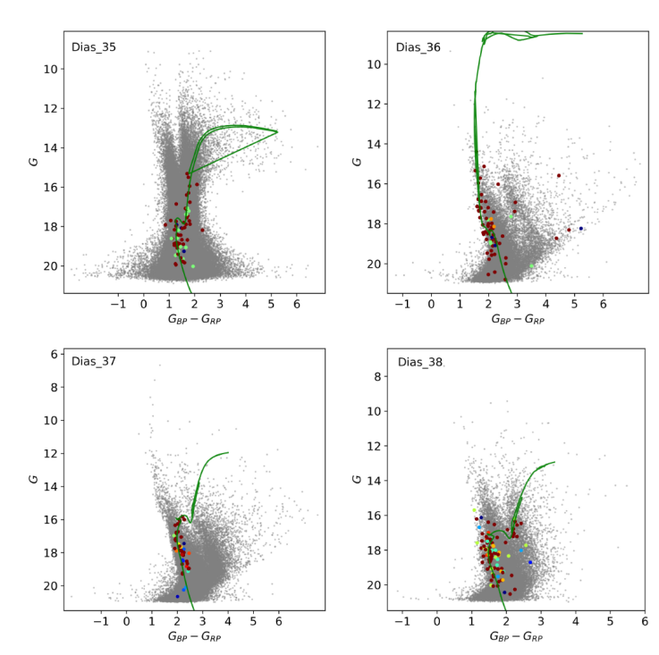
Fig. 2
Color-magnitude diagram with isochrone fitted for some of the discovered clusters studied. The color is proportional to the astrometric membership, where more red means a higher membership probability. The gray points correspond to field stars. The CMDs of all clusters in the sample are shown in Appendix. The color figure can be viewed online.
Color-magnitude diagram with isochrone fitted for some of the discovered clusters studied. The color is proportional to the astrometric membership, where more red means a higher membership probability. The gray points correspond to field stars. The CMDs of all clusters in the sample are shown in Appendix. The color figure can be viewed online.
From a quantitative perspective, these cases exhibit typical errors in the average astrometric parameters, as well as distances and ages, compared to the values reported in the literature, particularly those published in Dias et al. (2021), where we used the same isochrone fitting technique. As expected, the clusters with greater uncertainty in the distance and age parameters present a larger spread in the turn-off and main sequence.
-
Dias et al. (2021)MNRAS, 2021
Table 1 summarizes the positions, sizes, and astrometric parameters of these 28 discovered open clusters determined using stars with a membership probability greater than 0.50. The mean radial velocities are provided for 14 clusters using the radial velocity data given in the Gaia DR3 catalog. Table 2 provides the results of the fundamental parameters (distance, age, [Fe/H] and A V ) obtained by the isochrone fit given by the mean and standard deviation of the results of ten runs of the fitting procedure, as detailed in last section. In addition to the cluster parameters, all membership probabilities and individual stellar data are also made electronically available.
TABLE 1
MEAN ASTROMETRIC PARAMETERS FOR 28 DISCOVERED OPEN CLUSTERS
MEAN ASTROMETRIC PARAMETERS FOR 28 DISCOVERED OPEN CLUSTERS
| Field | Name |
RA ICRS [deg] |
DE ICRS [deg] |
R [arcmin] |
N |
pmRA [mas yr -1] |
e_pmRA [mas yr -1] |
pmDE [mas yr -1] |
e_pmDE [mas yr -1] |
P lx [mas] |
e_Plx [mas] |
RV [km s -1] |
e_RV [km s -1] |
NRV |
|---|---|---|---|---|---|---|---|---|---|---|---|---|---|---|
| 121.37+3.47 | Dias_12 | 9.2993 | 66.3245 | 12.681 | 79 | -1.540 | 0.227 | -0.006 | 0.163 | 0.159 | 0.087 | -91.057 | 2.089 | 2 |
| 123.93+1.43 | Dias_13 | 15.0612 | 64.3680 | 9.861 | 54 | -1.603 | 0.228 | -0.114 | 0.114 | 0.162 | 0.061 | … | … | 0 |
| 131.86+1.33 | Dias_14 | 33.1042 | 62.5949 | 19.458 | 141 | -0.921 | 0.238 | 0.092 | 0.302 | 0.213 | 0.056 | -60.781 | 0.830 | 2 |
| 137.69+3.88 | Dias_15 | 45.9315 | 62.9139 | 19.751 | 85 | -0.089 | 0.138 | 0.056 | 0.209 | 0.188 | 0.050 | -33.649 | 2.538 | 2 |
| 149.59+0.90 | Dias_16 | 61.9305 | 53.5426 | 14.053 | 52 | 0.116 | 0.244 | 0.326 | 0.121 | 0.161 | 0.043 | … | … | 0 |
| 151.63+3.36 | Dias_17 | 66.5584 | 53.4130 | 3.394 | 31 | 0.108 | 0.174 | -1.044 | 0.136 | 0.227 | 0.070 | … | … | 0 |
| 180.73-2.51 | Dias_18 | 84.2710 | 26.5927 | 6.774 | 43 | 0.340 | 0.138 | -0.306 | 0.186 | 0.220 | 0.076 | -11.718 | 2.078 | 2 |
| 184.89-1.74 | Dias_19 | 87.7687 | 23.6001 | 8.012 | 49 | 0.398 | 0.141 | -0.632 | 0.274 | 0.197 | 0.091 | … | … | 0 |
| 203.71+1.18 | Dias_20 | 99.5408 | 8.2739 | 17.297 | 44 | -0.167 | 0.146 | -0.377 | 0.163 | 0.209 | 0.049 | 39.631 | 1.380 | 5 |
| 213.07-2.23 | Dias_21 | 100.8634 | -1.2482 | 6.837 | 44 | -0.423 | 0.137 | 0.534 | 0.100 | 0.178 | 0.051 | … | … | 0 |
| 227.75-0.15 | Dias_22 | 110.0193 | -13.3799 | 11.545 | 40 | -0.647 | 0.083 | 0.751 | 0.097 | 0.226 | 0.035 | … | … | 0 |
| 245.93+1.16 | Dias_23 | 120.7232 | -28.0161 | 6.765 | 35 | -1.815 | 0.130 | 2.482 | 0.200 | 0.192 | 0.035 | 47.955 | 2.839 | 2 |
| 251.88-0.47 | Dias_24 | 122.8776 | -34.0747 | 8.613 | 45 | -2.482 | 0.092 | 3.008 | 0.109 | 0.167 | 0.026 | 96.460 | 3.521 | 5 |
| 251.52+2.00 | Dias_25 | 124.5981 | -32.1535 | 17.975 | 66 | -2.293 | 0.222 | 2.760 | 0.359 | 0.160 | 0.023 | 76.386 | 3.494 | 5 |
| 273.89-1.58 | Dias_26 | 140.2921 | -52.4072 | 7.759 | 40 | -3.598 | 0.222 | 2.928 | 0.135 | 0.115 | 0.049 | … | … | 0 |
| 292.34-4.88 | Dias_27 | 166.1039 | -65.0980 | 16.645 | 256 | -5.232 | 0.466 | 2.062 | 0.249 | 0.137 | 0.057 | 32.308 | 1.785 | 7 |
| 293.34-0.86 | Dias_28 | 171.5147 | -62.1815 | 4.021 | 50 | -6.135 | 0.243 | 1.207 | 0.162 | 0.280 | 0.040 | … | … | 0 |
| 318.06-0.46 | Dias_29 | 224.3485 | -59.3583 | 14.043 | 147 | -4.748 | 0.724 | -3.380 | 0.332 | 0.344 | 0.054 | -27.172 | 1.566 | 10 |
| 354.99+5.17 | Dias_30 | 258.0942 | -30.3556 | 5.505 | 32 | -3.817 | 0.287 | -5.791 | 0.301 | 0.084 | 0.055 | 2.528 | 2.009 | 3 |
| 16.28-2.81 | Dias_31 | 277.6833 | -16.1074 | 8.520 | 31 | -1.179 | 0.193 | -3.047 | 0.241 | 0.259 | 0.056 | … | … | 0 |
| 20.29-1.14 | Dias_32 | 278.2984 | -11.9047 | 8.905 | 148 | -0.304 | 0.242 | -1.854 | 0.291 | 0.261 | 0.079 | 5.205 | 5.335 | 4 |
| 22.76-0.25 | Dias_33 | 278.6223 | -9.3315 | 7.998 | 28 | -0.834 | 0.170 | -2.938 | 0.425 | 0.327 | 0.023 | -4.218 | 3.239 | 2 |
| 32.74-0.08 | Dias_34 | 283.1168 | -0.4266 | 4.022 | 41 | -1.626 | 0.106 | -4.295 | 0.087 | 0.217 | 0.032 | 51.251 | 1.468 | 6 |
| 26.61-3.98 | Dias_35 | 283.6507 | -7.5504 | 16.807 | 64 | -2.782 | 0.225 | -5.609 | 0.313 | 0.147 | 0.038 | … | … | 0 |
| 54.15+0.17 | Dias_36 | 292.4729 | 19.0487 | 3.783 | 66 | -2.595 | 0.157 | -5.523 | 0.181 | 0.211 | 0.065 | … | … | 0 |
| 60.57-0.19 | Dias_37 | 296.4799 | 24.1809 | 3.782 | 44 | -1.709 | 0.102 | -4.280 | 0.116 | 0.267 | 0.080 | … | … | 0 |
| 98.51+3.31 | Dias_38 | 324.2194 | 56.6787 | 11.981 | 98 | -2.526 | 0.255 | -2.044 | 0.120 | 0.103 | 0.044 | … | … | 0 |
| 98.51+3.31 | Dias_39 | 324.3774 | 57.0073 | 9.374 | 44 | -2.466 | 0.101 | -2.185 | 0.084 | 0.129 | 0.035 | … | … | 0 |
TABLE 2
RESULTS OF FUNDAMENTAL PARAMETERS OBTAINED FROM THE ISOCHRONE FIT
RESULTS OF FUNDAMENTAL PARAMETERS OBTAINED FROM THE ISOCHRONE FIT
| Field | Cluster |
Dist [pc] |
e_dist [pc] |
logt(age) | e_log(age) |
Av [mag] |
e_Av [mag] |
FeH [dex] |
e_FeH [dex] |
|---|---|---|---|---|---|---|---|---|---|
| 121.37+3.47 | Dias_12 | 6069 | 1506 | 8.939 | 0.405 | 4.010 | 0.395 | -0.181 | 0.063 |
| 123.93+1.43 | Dias_13 | 3120 | 1180 | 8.770 | 0.731 | 3.064 | 0.349 | -0.333 | 0.101 |
| 131.86+1.33 | Dias_14 | 3546 | 690 | 8.357 | 0.494 | 2.407 | 0.223 | -0.208 | 0.042 |
| 137.69+3.88 | Dias_15 | 6403 | 1310 | 9.027 | 0.218 | 2.743 | 0.283 | -0.181 | 0.130 |
| 149.59+0.90 | Dias_16 | 3834 | 760 | 8.805 | 0.312 | 2.616 | 0.183 | -0.361 | 0.116 |
| 151.63+3.36 | Dias_17 | 3137 | 615 | 8.225 | 0.763 | 2.480 | 0.220 | -0.295 | 0.034 |
| 180.73-2.51 | Dias_18 | 3733 | 413 | 8.659 | 0.238 | 2.403 | 0.241 | -0.263 | 0.101 |
| 184.89-1.74 | Dias_19 | 5193 | 557 | 8.787 | 0.723 | 2.545 | 0.164 | -0.269 | 0.137 |
| 203.71+1.18 | Dias_20 | 4678 | 761 | 8.882 | 0.197 | 2.197 | 0.187 | -0.304 | 0.097 |
| 213.07-2.23 | Dias_21 | 4295 | 225 | 7.730 | 0.209 | 1.973 | 0.058 | -0.227 | 0.088 |
| 227.75-0.15 | Dias_22 | 3504 | 236 | 8.327 | 0.430 | 1.614 | 0.118 | -0.206 | 0.074 |
| 245.93+1.16 | Dias_23 | 5563 | 545 | 9.210 | 0.292 | 1.246 | 0.305 | -0.183 | 0.053 |
| 251.88-0.47 | Dias_24 | 5769 | 705 | 8.179 | 0.863 | 1.676 | 0.225 | -0.194 | 0.121 |
| 251.52+2.00 | Dias_25 | 4626 | 286 | 7.885 | 0.416 | 1.356 | 0.096 | -0.262 | 0.056 |
| 273.89-1.58 | Dias_26 | 5246 | 1649 | 8.519 | 0.456 | 2.777 | 0.504 | -0.149 | 0.231 |
| 292.34-4.88 | Dias_27 | 6346 | 878 | 9.476 | 0.228 | 2.072 | 0.201 | -0.088 | 0.066 |
| 293.34-0.86 | Dias_28 | 3489 | 696 | 6.969 | 0.444 | 2.889 | 0.139 | 0.083 | 0.079 |
| 318.06-0.46 | Dias_29 | 2457 | 373 | 8.070 | 0.754 | 4.064 | 0.111 | 0.156 | 0.031 |
| 354.99+5.17 | Dias_30 | 10691 | 3453 | 10.022 | 0.216 | 2.056 | 0.506 | 0.195 | 0.061 |
| 16.28-2.81 | Dias_31 | 3966 | 788 | 9.052 | 0.216 | 2.838 | 0.177 | 0.217 | 0.078 |
| 20.29-1.14 | Dias_32 | 4783 | 240 | 8.823 | 0.055 | 4.050 | 0.101 | 0.332 | 0.062 |
| 22.76-0.25 | Dias_33 | 3537 | 455 | 8.667 | 0.569 | 3.956 | 0.121 | 0.342 | 0.106 |
| 32.74-0.08 | Dias_34 | 3077 | 655 | 8.414 | 0.259 | 4.039 | 0.101 | 0.409 | 0.131 |
| 26.61-3.98 | Dias_35 | 5539 | 1074 | 9.577 | 0.049 | 1.425 | 0.063 | 0.219 | 0.074 |
| 54.15+0.17 | Dias_36 | 3893 | 555 | 7.007 | 0.689 | 3.633 | 0.106 | 0.102 | 0.069 |
| 60.57-0.19 | Dias_37 | 2903 | 774 | 8.951 | 0.761 | 3.709 | 0.404 | 0.074 | 0.049 |
| 98.51+3.31 | Dias_38 | 6826 | 1583 | 8.962 | 0.101 | 2.897 | 0.225 | -0.178 | 0.111 |
| 98.51+3.31 | Dias_39 | 5181 | 1027 | 8.611 | 0.621 | 2.782 | 0.313 | -0.246 | 0.036 |
5. DISCUSSION
The superposition of known open clusters in their projections on the sky can occur with some frequency, especially in regions rich in stars and clusters. However, depending on the situation, the identification of new clusters can be obscured by a denser open cluster in the field, as for example discussed by Hunt & Reffert (2023) for the case of HSC_2382 in the field of IC_2662, as well as new star clusters discovered in the field of the open cluster NGC_5999 by Ferreira et al. (2019), and around NGC_6649 by Gao (2024).
-
Hunt & Reffert (2023)A&A, 2023
-
Ferreira et al. (2019)MNRAS, 2019
-
Gao (2024)MNRAS, 2024
In this work, five discovered clusters are located in the field of known open clusters. Our investigation of the cross-match with the clusters published in Hunt’s catalog, as well as the mean astrometric parameters and distance and age estimated from the isochrone fit, ensure that this is not a rediscovery of the same known open cluster. The new clusters in the same field of known clusters are the following: Dias_22 is about 13 arcmin from Haffner_6, Dias_23 is 12 arcmin from UBC_640, Dias_31 is 19 arcmin from Ruprecht_171, Dias_32 16 arcmin from Ruprecht_143 and Dias_34 is situated about 8 arcmin from the center of HSC 320.
Dias_38 and Dias_39 are two OCs found in the same investigated field with angular separation of 20 arcmin. In Figure 3 the sky map and the CMD of the investigated field 98.51 + 3.31 of one degree square are given with the 98 and 44 member stars of OC Dias_38 and Dias_39 superimposed in green and blue, respectively. As can be seen in Table 1 there is no significant difference in the astrometric parameters, but according to the results of our isochrone fit, over-plotted on the CMD in Figure 3, the clusters have about the same age. However, Dias_38 is about 1500 pc more distant than Dias_39. Unfortunately, we did not find members with determined radial velocity that would be useful for determining the Galactic orbits of the objects. This could be an interesting case for checking the possibility that the two are binary clusters. We understand that these cases need further confirmation.
Thumbnail
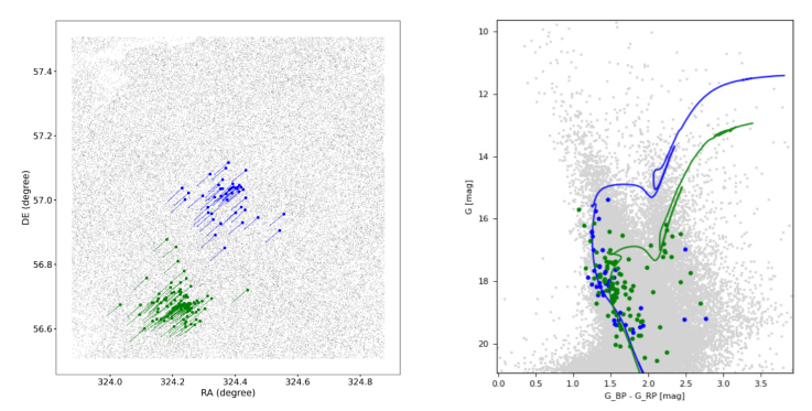
Fig. 3
Sky map and color-magnitude diagram of the stars in the field 98.51 + 3.31 with the member stars of the clusters Dias_38 and Dias_39 plotted in green and blue, respectively. The length of the vectors are presented in arbitrary units. The isochrones in the CMD are those with results given in the Table 2. The color figure can be viewed online.
Sky map and color-magnitude diagram of the stars in the field 98.51 + 3.31 with the member stars of the clusters Dias_38 and Dias_39 plotted in green and blue, respectively. The length of the vectors are presented in arbitrary units. The isochrones in the CMD are those with results given in the Table 2. The color figure can be viewed online.
Finally, we point out that Dias_30 is the older and more distant open cluster candidate of the sample and it is also among the oldest and most distant in the list of known open clusters. The CMD, presented in Figure 5, shows that the members selected by the HDBSCAN algorithm turn away from the main sequence towards the giant branch. The absence of a defined main sequence due to possible members beyond the limiting magnitude of the Gaia DR3 catalog results in poor parameter estimates by our code. However, we opted to maintain this new candidate in our list, since it is at the limit of detection of the Gaia DR3 data.
6. CONCLUSIONS
This paper presents the first results of the ongoing project to search for open clusters using a clustering algorithm applied to Gaia data. We report 28 new open clusters in our Galaxy discovered by applying the HDBSCAN algorithm to Gaia DR3 data in fields of star formation from the catalog published by Avedisova (2002).
-
Avedisova (2002)ARep, 2002
We determined the astrometric membership probability of the stars in each field using the HDB-SCAN algorithm applied in a variational fashion, which eliminates the need for initial assumptions about the tuning parameters of the method.
For all clusters, we determined mean proper motions and parallaxes, as well as the fundamental parameters (d, log(t), A V ) and [Fe/H]), using our non-subjective multidimensional global optimization tool to fit theoretical isochrones to Gaia DR3 photometric data.
We were able to obtain the mean radial velocity for 14 open clusters using radial velocity data published in the Gaia DR3 catalog.
Surprisingly, we found Dias_30 among the oldest and most distant in the list of the known open clusters in the Galaxy, making it an interesting case to be investigated further with deep data such as Euclid, LSST and ELT.
Finally, the results of this work indicate that there is still work to be done on open cluster discovery. Although the need for automated searches is evident, the use of clustering algorithms has not yet been exhausted as, depending on the technique, OCs with different characteristics are detected. Even HDBSCAN deserves to be tested with different tuning parameters in the search, mainly due to its efficiency and speed.
Acknowledgements
We thank the referee for the valuable suggestions that improved the quality of the paper. W.S.Dias is Bolsista FAPEMIG - CNPq - Brasil (processo BPQ-06608-24) and acknowledges FAPESP (fellowship 2024/15923-1) and CNPq (fellowship 310765/2020-0). H. Monteiro would like to thank FAPEMIG grants APQ-02030-10 and CEX-PPM-00235-12. This research was performed using the facilities of the Laboratório de Astrofísica Computacional da Universidade Federal de Itajubá (LAC-UNIFEI). This work has made use of data from the European Space Agency (ESA) mission Gaia (http://www.cosmos.esa.int/Gaia), processed by the Gaia Data Processing and Analysis Consortium (DPAC, http://www.cosmos.esa.int/web/Gaia/dpac/consortium). We employed catalogs from CDS/Simbad (Strasbourg) and Digitized Sky Survey images from the Space Telescope Science Institute (US Government grant NAG W-2166).
References
- Avedisova, V. S. 2002, ARep, 46, 193, https://doi.org/10.1134/1.1463097 Links
- Bonnarel, F., Fernique, P., Bienayme, O., et al. 2000, A&AS, 143, 33, https://doi.org/10.1051/aas:2000331 Links
- Bressan, A., Marigo, P., Girardi, L., et al. 2012, MNRAS, 427, 127, https://doi.org/10.1111/j.1365-2966.2012.21948.x Links
- Campello, R. J. G., Moulavi, D., & Sander, J. 2013, Density-Based Clustering Based on Hierarchical Density Estimates in Advances in Knowledge Discovery and Data Mining 17th Pacific-Asia Conference, PAKDD, ed. J. Pei, V. Tseng, L. Cao, H. Motoda, & G. Xu, 160-172, https://doi.org/10.1007/978-3-642-37456-2_14 Links
- Campello, R. J. G. B., Moulavi, D., Zimek, A., & Sander, J. 2015, ACM Transactions on Knowledge Discovery from Data (TKDD), 10, 1, https://doi.org/10.1145/2733381 Links
- Cantat-Gaudin, T. & Anders, F. 2020, A&A, 633, 99, https://doi.org/10.1051/0004-6361/201936691 Links
- Capitanio, L., Lallement, R., Vergely, J. L., Elyajouri, M., & Monreal-Ibero, A. 2017, A&A, 606, 65, https://doi.org/10.1051/0004-6361/201730831 Links
- Castro-Ginard, A., Jordi, C., Luri, X., et al. 2020, A&A, 635, 45, https://doi.org/10.1051/0004-6361/201937386 Links
- Castro-Ginard, A., Jordi, C., Luri, X., Cantat-Gaudin, T., & Balaguer-Nuñez, L. 2019, A&A, 627, 35, https://doi.org/10.1051/0004-6361/201935531 Links
- Dias, W. S., Alessi, B. S., Moitinho, A., & Lepine, J. R. D. 2002, A&A, 389, 871, https://doi.org/10.1051/0004-6361:20020668 Links
- Dias, W. S., Monteiro, H., Lepine, J. R. D., et al. 2018, MNRAS, 481, 3887, https://doi.org/10.1093/mnras/sty2341 Links
- Dias, W. S., Monteiro, H., Moitinho, A., et al. 2021, MNRAS, 504, 356, https://doi.org/10.1093/mnras/stab770 Links
- Ester, M., Kriegel, H.-P., Sander, J., & Xu, X. 1996, in Proc. of 2nd International Conference on Knowledge Discovery and Data Mining (KDD-96), 226 Links
- Evans, D. W., Riello, M., De Angeli, F., et al. 2018, A&A, 616, 4, https://doi.org/10.1051/0004-6361/201832756 Links
- Ferreira, F. A., Santos, J. F. C., Corradi, W. J. B., Maia, F. F. S., & Angelo, M. S. 2019, MNRAS, 483, 5508, https://doi.org/10.1093/mnras/sty3511 Links
- Gao, X. 2024, MNRAS, 527, 1784, https://doi.org/10.1093/mnras/stad3358 Links
- Hao, C. J., Xu, Y., Wu, Z. Y., et al. 2022, A&A, 660, 4, https://doi.org/10.1051/0004-6361/202243091 Links
- He, Z., Li, C., Zhong, J., et al. 2022, ApJS, 260, 8, https://doi.org/10.3847/1538-4365/ac5cbb Links
- Hunt, E. L. & Reffert, S. 2021, A&A, 646, 104, https://doi.org/10.1051/0004-6361/2020239341 Links
- ______ 2023, A&A, 673, 114, https://doi.org/10. 1051/0004-6361/202346285 Links
- ______ 2024, arXiv e-prints, arXiv:2403.05143, https://doi.org/10.1051/0004-6361/202348662 Links
- Jaehnig, K., Bird, J., & Holley-Bockelmann, K. 2021, ApJ, 923, 129, https://doi.org/10.3847/1538-4357/ac1d51 Links
- Kharchenko, N. V., Pakulyak, L. K., & Piskunov, A. E. 2003, ARep, 47, 263, https://doi.org/10.1134/1.1568131 Links
- Kounkel, M. & Covey, K. 2019, AJ, 158, 122, https://doi.org/10.3847/1538-3881/ab339a Links
- Kounkel, M., Covey, K., & Stassun, K. G. 2020, AJ, 160, 279, https://doi.org/10.3847/1538-3881/abc0e6 Links
- Krone-Martins, A. & Moitinho, A. 2014, A&A, 561, 57, https://doi.org/10.1051/0004-6361/201321143 Links
- Liu, L. & Pang, X. 2019, ApJS, 245, 32, https://doi.org/10.3847/1538-4365/ab530a Links
- Monteiro, H. & Dias, W. S. 2019, MNRAS, 487, 2385, https://doi.org/10.1093/mnras/stz1455 Links
- Monteiro, H., Dias, W. S., & Caetano, T. C. 2010, A&A, 516, 2, https://doi.org/10.1051/0004-6361/200913677 Links
- Monteiro, H., Dias, W. S., Hickel, G. R., & Caetano, T. C. 2017, NewA, 51, 15, https://doi.org/10.1016/j.newast.2016.08.001 Links
- Monteiro, H., Dias, W. S., Moitinho, A., et al. 2020, MNRAS, 499, 1874, https://doi.org/10.1093/mnras/staa2983 Links
- Pedregosa, F., Varoquaux, G., Gramfort, A., et al. 2011, Journal of Machine Learning Research, 12, 2825, http://jmlr.org/papers/v12/pedregosa11a.html Links
- Pera, M. S., Perren, G. I., Moitinho, A., Navone, H. D., & Vazquez, R. A. 2021, A&A, 650, 109, https://doi.org/10.1051/0004-6361/202040252 Links
- Sim, G., Lee, S. H., Ann, H. B., & Kim, S. 2019, JKS, 52, 145, https://doi.org/10.5303/JKAS.2019.52.5.145 Links
APPENDIX
APPENDIX
Color-magnitude diagram with isochrones fitted for the discovered clusters.
Thumbnail
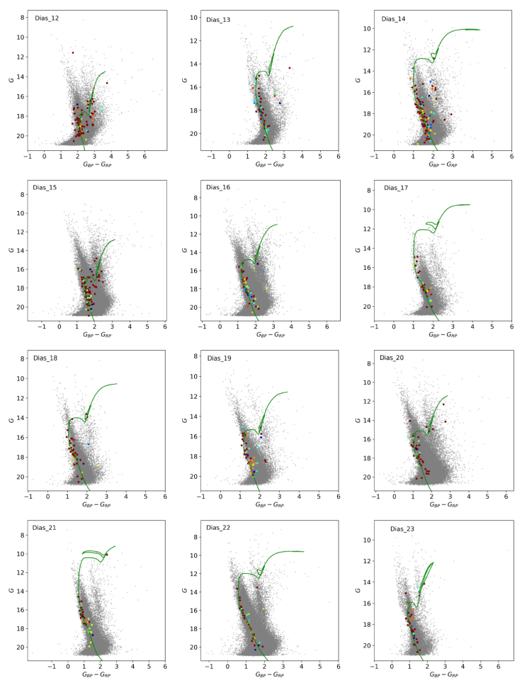
Fig. 4
Color-magnitude diagram with isochrone fitted for the discovered clusters studied. The color is proportional to the astrometric membership, where more red means higher membership probability. The gray points correspond to field stars. The color figure can be viewed online.
Color-magnitude diagram with isochrone fitted for the discovered clusters studied. The color is proportional to the astrometric membership, where more red means higher membership probability. The gray points correspond to field stars. The color figure can be viewed online.
Thumbnail
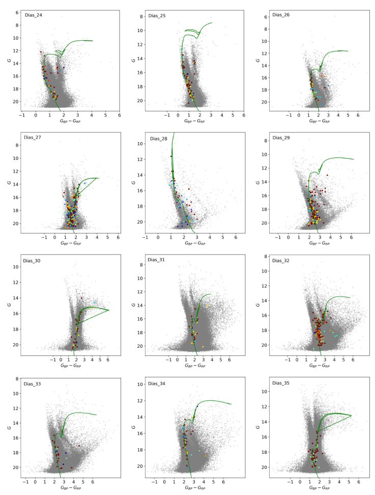
Fig. 5
Same as Figure 4. The color figure can be viewed online.
Same as Figure 4. The color figure can be viewed online.
Thumbnail
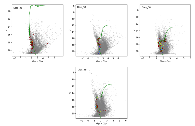
Fig. 6
Same as Figure 4. The color figure can be viewed online.
Same as Figure 4. The color figure can be viewed online.