


 nueva página del texto (beta)
 Inglés (pdf)
 Artículo en XML
 Referencias del artículo
 Enviar artículo por email
 Citado por SciELO
  Similares en
SciELO
Similares en
SciELO 
 Permalink
1. Introduction
The Calar Alto Void Integral-field Treasury Survey (CAVITY Pérez et al. 2024) is an ongoing legacy project by the Calar Alto Observatory. Its goal is to collect detailed observations of ≈300 galaxies found in empty spaces of the Universe, known as voids, using the PMAS/PPaK instrument located on the 3.5m telescope at Calar Alto, the same used by the CALIFA project (e.g. Sánchez et al. 2012). CAVITY aims to understand how galaxies grow and what their stars and gas are like in these lonely parts of space, helping to estimate how being in such an empty environment affects the birth and growth of a galaxy.
The CAVITY project has already observed a total of 208 galaxies during the last three years, completing ≈70% of the foreseen sample. Early exploration using SDSS single spectroscopy (York et al. 2000) of the entire parent sample from which this observed sub-sample was drawn has already provided some interesting results. Domínguez-Gómez et al. (2023b) managed to trace back the history of star formation in galaxies living in different environments, like clusters, filaments and walls of galaxies, and the voids. They found that galaxies in voids take longer to build up their mass. In Domínguez-Gómez et al. (2023a) it was explored how the stellar metallicity of galaxies changes depending on their location. They discovered that galaxies in voids tend to have slightly less metals compared to those in denser areas, especially the smaller galaxies. In particular, they found a noticeable difference in metal content between void galaxies and those in clusters.
More recently, Conrado et al. (2024) delved deeper into the characteristics of galaxies in voids by exploring, for the first time, the spatially resolved properties of the stellar populations in a sub-sample of the CAVITY dataset, including the mass, age, star formation rate (SFR), and specific star formation rate (sSFR), both over-all and relative to their distance from the center of the galaxy. They compared their results to similar analyses of galaxies located in denser environments, like filaments and walls, using data from the CALIFA survey. They found that galaxies in voids tend to have lower stellar mass surface density, younger ages, and higher values of SFR and sSFR. Many of these differences appear in the outer parts of spiral galaxies (R > 1Re), which are younger and have higher sSFR than galaxies in filaments and walls, indicating that their disks are less evolved. Large variations also occur for early-type spirals, which points to a slower transition from star-forming to quiescent galaxies in voids.
Following a similar approach adopted in previous Integral Field Spectroscopy (IFS) galaxy surveys (e.g. Sánchez et al. 2022), we describe in this paper the data products of the analysis for the CAVITY IFS dataset using the pyPipe3D pipeline (Lacerda et al. 2022). pyPipe3D is a recently updated version of Pipe3D fully coded in Python. The Pipe3D pipeline makes use of the routines and algorithms included in the FIT3D package (Sánchez et al. 2016c), with the main goal of extracting the properties of the ionized gas and the stellar component of an observed galaxy using its IFS data in the optical range. Pipe3D has been extensively used to explore the data from different surveys: e.g., CALIFA (Sánchez-Menguiano et al. 2016; Espinosa-Ponce et al. 2020), SAMI (Sánchez et al. 2019b), AMUSING++ (Sánchez-Menguiano et al. 2018; López-Cobá et al. 2020) and MaNGA (Sánchez et al. 2018, 2022).
This article is organized as follows: § 2 provides an overview of the dataset under investigation, including a brief summary of the observations and data reduction process; § 3 outlines the selection criteria and the main properties of the sample; the analysis performed on the data is described in § 4, including a summary of the main procedures included in the adopted Pipeline (§ 4.1), a description of the procedures to derive the provided physical quantities (§ 4.3), and how the integrated and characteristics properties are estimated (§ 4.4); the results of this analysis are presented in § 5, including a description of the data model adopted for the final delivered data products (§ 5.1), and the catalog of parameters extracted for each galaxy (§ 5.2); an example of the use of the derived parameters, exploring the global intensive and extensive relations that rule star-formation in galaxies, is included in § 5.3; finally, the summary and conclusions of this study are presented in § 6.
Throughout this study, when necessary, we assumed a standard Λ Cold Dark Matter cosmology with the following parameters: H 0=71 km/s/Mpc, Ω M =0.27, ΩΛ=0.73.
2. Observations and data reduction
Observational data were acquired using the 3.5m telescope located at the Calar Alto Observatory, employing the Potsdam Multi-Aperture Spectrometer (PMAS) in its PPaK configuration, as detailed by Roth et al. (2005) and Kelz et al. (2006), respectively. The PPaK configuration incorporates a 382 fiber bundle, effectively covering a field of view measuring 74′′ by 64′′. Each fiber, positioned in an hexagonal layout, possesses a diameter of 2.7′′ on the sky, achieving a filling factor of 60%. This configuration is augmented by six peripheral bundles, each comprising six fibers, dedicated to sampling the sky background at the edges of the field of view. Through the application of a three-position dithering pattern, the filling factor is enhanced to 100%, resulting in data cubes with dimensions of 78 by 73 pixels, where each pixel corresponds to a spatial area of 1′′ by 1′′. These observations were conducted in the V500 low-resolution mode, yielding a resolution of approximately R ≈850 at 5000 Å with a full width at half maximum (FWHM) of roughly 6 Å. The wavelength span for this observational mode extends from 3745 to 7500 Å, with a spectral sampling interval of 2 Å.
The data reduction pipeline of the CAVITY project is built on the techniques and procedures developed to reduce the data from the IFS observations (Sánchez 2006) and, in particular, those implemented to handle the data from the CALIFA survey (Sánchez et al. 2016a), introducing the required modifications to meet the particular needs of the CAVITY project. The pivotal steps included in the pipeline are summarized here: (i) pre-processing of the raw data to consolidate reads from different amplifiers into a single frame, removing bias, adjusting for gain, and cleaning cosmic rays; (ii) identification and tracing of spectra from various fibers on the CCD, determining the FWHM of the projected spectra along both dispersion and cross-dispersion axes; (iii) spectra extraction using the previously estimated trace and widths, with a removal of stray-light effects; (iv) wavelength calibration and resampling to achieve a linear wavelength scale (2Å per spectral pixel); (v) homogenization of spectral resolution across wavelengths, setting a final resolution of FWHM = 6Å; (vi) correction for differential fiber-to-fiber transmission; (vii) flux calibration of the spectra; separation of science fibers (covering the central hexagonal area) from sky-sampling fibers, and subtraction of a night-sky spectrum for each dither point; (ix) combining the three dither points into a single spectral frame with an associated position table; (x) generation of a final data cube using the image reconstruction procedure described in García-Benito et al. (2015), in which the X and Y coordinates correspond to the location in the sky and the Z coordinate to the wavelength. Pérez et al. and García-Benito et al. are preparing a more comprehensive discussion of this pipeline, which will be detailed in the upcoming CAVITY presentation paper and DR1 paper.
3. Sample
The CAVITY project mother sample includes 4866 galaxies located within 15 specifically chosen voids, as identified in the comprehensive void galaxy catalog by Pan et al. (2012), which catalogued 79,947 galaxies across 1,055 voids. These 15 voids were intentionally selected to represent a variety of sizes and dynamical states. The galaxies within this primary sample are part of the nearby Universe, with redshift values between 0.005 and 0.05, and cover a broad spectrum of masses, ranging from 108.5 to 1011 M⊙. The mass estimates for these galaxies were derived using the mass-to-light ratio from the color technique, as detailed by McGaugh & Schombert (2014). To be included in the sample, galaxies had to meet specific criteria: they must be located within 80% of the effective radius of their respective void; each void should have at least 20 galaxies along its radius for adequate sampling; and the galaxies’ distribution in right ascension must facilitate year-round observability.
This sample is far too large to be observable in a reasonable time. Like in the case of other IFS (e.g. CALIFA, MaNGA Sánchez et al. 2012), we used that sample as a pool of possible targets from which the actual galaxies to be observed were picked randomly according to their visibility on the allocated nights. In this way the observed sample should be a randomly selected sub-sample of the mother sample, being completely representative of the sample from which it was selected. This statement should be checked a posteriori, characterizing the possible deviations introduced during the object picking and observing process. Based on the range of parameters to be sampled it was estimated that observing ≈20 galaxies per void should be enough to achieve the goals of the project. Thus, the final observed sample is foreseen to comprise a total of ≈300 galaxies. The full procedure and the details of the properties for the foreseen observed sample was described in detail in the CAVITY presentation article (Pérez et al. 2024).
The sample analyzed in this study comprises 208 galaxies (i.e., ≈2/3 of the finally foreseen sample). Of them, 199 correspond to all the galaxies observed by the CAVITY project up to November 2023. Nine additional galaxies were extracted from the Voids Galaxy Survey (VGS) by Kreckel et al. (2011). These galaxies were observed using an identical instrument and settings as the CAVITY project during 2019 and 2020, effectively acting as a preliminary study. Of them, four targets already fulfill the CAVITY selection criteria, being part of the mother sample. On the contrary, the remaining five are not directly associated with any of the voids identified in the CAVITY project. Nevertheless, they were all included in our analysis. Finally, we should highlight that we are not distributing the full analyzed dataset, but only those galaxies included in the CAVITY DR1. The remaining data products will be liberated in the successive data releases of the project.
To illustrate which kind of galaxies are explored by the CAVITY project we compare their properties with those of galaxies covered by previous surveys, in particular their absolute magnitudes, colors and morphology. To do so we derive the synthetic magnitudes in the restframe directly from the reduced data cubes by convolving the redshifted SDSS-filters (Gunn et al. 2006) with the data cubes and applying the zero-point corresponding to the AB-photometric system. Then, using the standard cosmology, and without any K-correction, we derive the corresponding absolute magnitudes. Finally, following Conrado et al. (2024) we adopted the morphological classification provided by Domínguez Sánchez et al. (2018). To assign a Hubble classification, we utilized the T-Type parameter described by de Vaucouleurs (1963), separating between E and S0 following the prescriptions described in Domínguez Sánchez et al. (2018, 2022).
Figure 1 presents the color-magnitude diagram (CMD), g − r color against the r-band absolute magnitude, for the analyzed sub-sample. For comparison purposes we include the same distibution for the extended CALIFA sample (eCALIFA, Sánchez et al. 2023b) and a sub-sample of galaxies extracted from the NASA Sloan Atlas (SDSS-NSA, Blanton et al. 2017) that resembles a diameter selected sub-sample at the redshift footprint of eCALIFA (Sánchez et al. 2023b). It is evident that while the eCALIFA sample effectively spans through the CMD, covering a similar range of magnitudes and colors as a diameter selected sample at a similar redshift, the CAVITY sub-sample covers a much narrower range of magnitudes and colors. Low-luminosity (Mr >-18 mag) and extremely red objects (g − r >0.8 mag), are practically absent in the analyzed sub-sample. If we compare these distributions with those shown in Conrado et al. (2024), comparing with the CAVITY mother sample, it seems that the origin of the bias is in the observed sub-sample, not in the original selection.
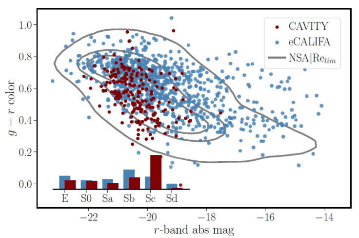
Fig. 1 Distribution in the g − r vs. r−band absolute magnitude diagram of the CAVITY galaxies (maroon solid-circles), compared to the same distribution for eCALIFA galaxies (blue solid-circles) and a sub-sample of SDSS-NSA galaxies selected using the same diameter, magnitude and redshift range as the eCALIFA compilation (grey contours). Each successive contour encircles a 95%, 65% and 40% of the SDSS-NSA galaxies. The bottom-left inset shows the morphological distribution of the CAVITY and eCALIFA galaxies. The color figure can be viewed online.
Additional differences are found in the morphologi-cal distribution, included as an inset in Figure 1. As already noticed by Conrado et al. (2024) for the CAVITY project, and in previous explorations of the properties of galaxies in Voids (e.g. Rojas et al. 2004; Kreckel et al. 2011), there is an excess of late-type spirals, in particular Sc, when comparing to field galaxies. This is true, even considering that eCALIFA has an over-representation of earlier type spirals, Sb-type (e.g. Sánchez et al. 2023b). Another difference is the apparent lack of Sd galaxies in the CAVITY sample. However, we should be cautious before drawing a clear conclusion in this regard, as a possible bias against this particular morphological type in the classification presented by Domínguez Sánchez et al. (2018) has been reported.
4. Analysis
Following the methodologies outlined by Sánchez et al. (2022, 2024a), we embarked on a detailed examination of our dataset to uncover the core features and overall properties of each galaxy within it. By leveraging the pyPipe3D pipeline on every data cube, we were able to discern the spatially resolved characteristics as well as the integrated aspects of these cosmic structures. This process involved the careful analysis of the outputs of the pipeline to distill a variety of physical measurements.
In this summary, we briefly outline the essence of our analytical process and the main findings derived from it. For a more detailed discussion and to avoid redundancy, we refer readers to our earlier works, particularly those by Sánchez et al. (2016b, 2022, 2024a), where we explore these topics in greater depth.
4.1. pyPipe3D Analysis
In our analysis, we employ pyPipe3D (Lacerda et al. 2022), an updated version of the Pipe3D pipeline (Sánchez et al. 2016b). This version has been recoded in Python, leveraging the advanced computational capabilities of this programming language to enhance performance, streamline the analysis sequence, and address any bugs identified in previous versions. Pipe3D is a robust and well-established tool, extensively applied in the analysis of Integral Field Spectroscopy (IFS) data across a wide array of data sets. Notably, it has contributed to significant insights within the CALIFA survey (e.g., Cano-Díaz et al. 2016a; Espinosa-Ponce et al. 2020), the MaNGA project (e.g., Ibarra-Medel et al. 2016; Barrera-Ballesteros et al. 2018; Sánchez et al. 2019a; Bluck et al. 2019; Sánchez-Menguiano et al. 2019), the SAMI Galaxy Survey (e.g., Sánchez et al. 2019b), and the AMUSING++ compilation (Sánchez-Menguiano et al. 2018; López-Cobá et al. 2020).
Furthermore, the efficiency and accuracy of the pipeline have been rigorously vetted through analyses involving mock data sets and specialized simulations designed around hydrodynamical models (Guidi et al. 2018; Ibarra-Medel et al. 2019; Sarmiento et al. 2023). Here, we provide only a concise summary of the functionality of the code to prevent duplicate content.
4.1.1. Spatial Binning/Tessellation
The pyPipe3D pipeline uses the pyFIT3D package to automatically analyze each data cube. To get accurate results for the stellar population analysis, it is important to increase the signal-to-noise ratio (S/N). This is done by grouping nearby pixels together in a process called spatial binning, which pyPipe3D does in a way that keeps the original light pattern of the galaxy as intact as possible (see Sánchez et al. 2016c; Lacerda et al. 2022, for more details). After binning, the software analyzes these grouped pixels to learn about the properties of the stellar population and the ionized gas in each region of the galaxy.
4.1.2. Stellar Population Analysis
As we mentioned before, each grouped (or binned) spectrum is analyzed by pyFIT3D. This part of the process separates the light coming from stars from the light coming from ionized gas in each part of the galaxy. To estimate the spectra corresponding to the stellar population, pyFIT3D creates a model using a mix of different single stellar populations (SSP) templates from the MASTAR_SLOG library. This library has 273 templates, covering 39 different ages of stars (from 1 Myr to 13.5 Gyr, following a logarithm scale) and 7 values of metallicity (Z/Z ⊙ = 0.006, 0.029, 0.118, 0.471, 1, 1.764, 2.353). This library was selected from a large set of SSP templates created with an updated version the GALAXEV stellar population synthesis code (Bruzual & Charlot 2003), adopting a Salpeter initial mass function (Salpeter 1955) and using the PARSEC isochrones (Bressan et al. 2012) and the MaStar empirical stellar library (Yan et al. 2019) as basic ingredients. For more details on how we picked these particular subset of templates, see Appendix A, in Sánchez et al. (2022).
Before making the model, the SSP templates are adjusted to match the speed at which the galaxy is moving towards or away from us (systemic velocity) and how spread out the speeds of the stars in the galaxy are (velocity dispersion). We also consider how dust in the galaxy might be dimming the star light (dust attenuation) using the formula from Cardelli et al. (1989).
After adjusting the SSPs for kinematics, spread, and dust effects, we fit them to the spectra of the galaxy. This is done through a step-by-step process, as described in Sánchez et al. (2016c) and Lacerda et al. (2022), where we keep adding or removing templates to get the best match. To do so we perform a linear combination of the adjusted templates, starting with all the templates in the library. Then, from each iteration all those templates that contribute with a negative coefficient are removed from the library. The goal is to mix only those templates that contribute with a positive coefficient. The procedure stops once this goal is reached. Several iterations are performed perturbing the original spectrum by the error, ending up with several (different) realizations of the fitting.
This iterative procedure is performed twice. First, a limited SSP library is adopted with just 12 templates selected to avoid degenerancies between the stellar parameters (age and metallicity) and non-linear parameters that describe the kinematics (velocity and velocity dispersion) and dust attenuation. This template is adopted in the exploration of these three non-linear parameters, performing a brute-force exploration of the space of parameters. Then, we fix these three parameters, readjust the full library according to them, and re-analyze the spectrum.
The average (standard-deviation) of the positive coefficients derived in each iteration described before weights the (error of the) contribution of each SSP to the observed spectrum. The sum of all the SSPs in the library weighted by those coefficients is the final model. This spectral model is then matched to the flux intensity in a specific part of the spectrum (5450-5550Å, which is in the range of what we call the V-band). In this procedure the strongest emission lines are first masked. Then, once their contribution is estimated as we will describe in the next section, it is removed from the original spectrum and the derivation of the stellar model is repeated. This procedure could be iterated several times until converging to a stable solution.
Finally pyFIT3D derives the luminosity- and mass-weighted parameters of the stellar population (LW and MW ) using the coefficients of the stellar decomposition, following equation (2) in Sánchez et al. (2024a). In essence an average of the logarithm values of the considered parameters is performed; that is, a geometrical average, weighted by the fraction of light (or mass) that each SSP contributes to the observed spectrum, multiplied by the corresponding value for the considered template. Also, the stellar mass across the considered aperture, using equation (3) in Sánchez et al. (2024a), is estimated by co-adding the mass in each analyzed spatial bin (§ 4.1.1). For each bin the stellar mass is derived by multiplying the dust corrected luminosity assigned to each SSP by the decomposition by its mass-to-light ratio (Υ S S P ), and then coadding for all the templates in the adopted library.
4.1.3. Emission Line Analysis
To estimate the observational properties of the ionized gas in the galaxy, the software first removes the light coming from the stars, using the best stellar spectrum model we described in the previous section. What is left is mostly light from the ionized gas. The code then looks at a particular emission line from the ionized gas11. Each of these emission lines gets fitted with a Gaussian function, in order to describe their shape, and to derive their velocity dispersion, systemic velocity and integrated flux.
This whole process, working out the stellar and ionized gas component, is iterated, refining each time both models. We use the best guess of the ionized gas spectrum to decontaminate the original spectrum and to create a spectrum that contains only light from the stars, and then we update our emission line model. We improve each model based on how well they fit the actual data we observe, judging the accuracy of the model by the best χ2.
The described process helps us understand the gas emission lines for each tessella or spatial bin. To dig deeper and learn about these emissions for individual pixels (spaxels), we have an extra step. We start by adjusting the best star model we found for each group of pixels to fit each individual pixel inside that group. This adjustment uses a special scaling factor (DZ, Cid Fernandes et al. 2013). Then, we subtract this adjusted star model from the original galaxy data to get a new data set that mainly includes gas emissions, along with some noise and residuals from the stellar model fitting.
Next, to estimate the properties of the gas emissions from this cleaned-up data, we use two approaches. (i) We fit Gaussian models to the brightest and more detectable emissions, as done before. (ii) We use a method that weighs different parts of the emissions to study both the strong and the faint ones, giving us a fuller picture. This second method not only tells us about the flux intensity (F el ), velocity (v el ), and velocity dispersion (σ el ) of these emissions but also measures how much light they emit compared to the background stellar component (i.e, the equivalent width, EW el ). The complete list of emission lines we looked at with this method were already published in Table 7 of Sánchez et al. (2024a).
4.1.4. Stellar Indices
Moreover, pyPipe3D calculates various stellar indices for each pixel group (voxel/tessella) in the data. First, it creates a stellar spectrum that is cleaned of any effect from gas emissions. This is done by removing the best gas emission model found earlier. Then, for each stellar index (which is a way of measuring specific features in the stellar spectrum), it looks at three different sections of the spectrum: (i) the main part where the stellar index is defined, and (ii) two side sections that help estimate the background light level. The list of stellar indices we specifically looked at in this study is included in Table 4 of Sánchez et al. (2024a).
4.1.5. Error Estimation
To make sure we know how accurate our findings are, we used the Monte Carlo (MC) method to estimate the errors for all the measured parameters. We take the original spectra for each spaxel (or each group of spaxels that have been binned together) and add random noise based on the uncertainties estimated during the data reduction. This gives us a set of 50 slightly altered versions of our original data.
Next, we go through the whole analysis process again for each of these tweaked versions. By looking at how the results vary across these different runs, we can get a good idea of how reliable our original measurements are. We say that the spread of these results (technically, their standard deviation) represents the error of our measurements.
It is important to note that whenever we remove the effects of gas emissions or stellar spectrum from our data to get a clearer look at either one, we also adjust our error estimates. This takes into account any extra uncertainty that might be added by our models of gas emissions or starlight. For a deeper dive into how we estimate these errors, refer to Lacerda et al. (2022).
4.2. Data Masks
For each measurement described before we derive the corresponding errors. In particular, the error of the flux intensity help us to decide which parts of the galaxy data present reliable information and which ones do not. Before we group pixels together (a process described in 4.1.1), we pick out the parts of the data where the flux intensity is stronger than the noise by at least a factor one. This helps us create a "selection mask" that guides us on where to focus our analysis of the properties in the galaxy.
We also make another mask to cover areas that might be messed up by foreground stars. We find these intrusive stars using the catalog of stars from Gaia DR312, that has mapped the positions and movements of billions of stars with unprecedented precision. We only consider stars from this catalog that have precise positions, meaning that their position is known five times more precisely than the uncertainty. Around each of these stars, we mask a circle with a radius of 2.5′′, avoiding the use of data within those circles.
4.3. Physical Quantities
The observational data extracted by pyPipe3D for each spaxel or tessella within the data cubes, encompassing both stellar populations and ionized gas emission lines, serve as the foundation for deriving more physical parameters. The methodologies employed to derive those parameters from the primary observational properties have been thoroughly elucidated in previous articles. For an indepth understanding of these procedures, readers are encouraged to consult the extensive discussions presented in Sánchez et al. (2021b, 2022, 2024a).
We show here the list of derived parameters and properties to avoid unnecessary
repetition: (i) stellar masses (M
⋆) and stellar mass surface density (Σ⋆), integrated along
the look-back time (i.e., the current values), the value for stellar populations
of a particular age, 𝒜⋆ (or metallicity, 𝒵⋆), of the
integrated up to a certain age of the Universe (i.e. the mass assembly history,
MAH); star-formation at a certain time (SFRssp,t), obtained as the
numerical derivative of the MAH, thus based on the stellar population analysis;
(iii) chemical enrichment history, i.e., the cummulative metallicity evaluated
up to a certain cosmological time ([Z/H]
t
); (iv) the time-scales at which a certain amount of the current
accumulated mass is formed (T% e.g., T80, time at which 80% of the stellar mass
was formed); (v) the metallicity at those time scales (a_ZH_T%); (vi) line
ratios that are commonly utilized to ascertain the characteristics of the
ionizing sources and to understand the physical properties of the ionized gas,
including [O II]/Hβ, [O III]/Hβ, [O
I]/Hα, [N II]/Hα, [S
II]/Hα, and Hα/Hβ; (vii)
the ionized gas dust attenuation (AV,gas) derived from the
Hα/Hβ-line ratio; oxygen and nitrogen
abundances and ionization parameter; a total of 28 oxygen abundances, 3 nitrogen
abundances and 4 ionization parameter estimations have been included using
different calibrators (the complete list is included in Appendix D and Table 15
of Sánchez et al. 2022); (ix) ionized gas
electron density n
e
; (x) star-formation rate derived from the dust-corrected Hα luminosity
(SFR), and the corresponding SFR surface density (ΣSFR); (xi)
molecular gas mass (M
mol) derived from the dust attenuation (based on the Hα/Hβ ratio,
i.e., A
V,gas
), following Barrera-Ballesteros et al.
(2020) and Barrera-Ballesteros et al.
(2021), and the corresponding surface density (Σmol); and
finally (xii) velocity to velocity dispersion ratio
We should note that, when required the Salpeter (1955) initial mass function is assumed through all the calculations.
4.4. Integrated, Aperture Limited and Characteristic Properties
The analysis we have conducted provides a range of parameters for every individual spaxel, tessella, or at a certain distance from the galaxy center. Using these data, we calculate the values of various extensive properties (like stellar mass, M ⋆, or SFR) at different sizes of areas: the whole galaxy, within 1 effective radius (Re), or in a central region (1.5′′ in diameter). For properties that do not depend on the size of the area (intensive properties), such as star density (Σ⋆), oxygen abundance, or the explored stellar indices, we estimate the azimuthal average values at various distances from the galaxy center. This method follows the approach outlined in previous research by Sánchez (2020), Sánchez et al. (2021b), and Barrera-Ballesteros et al. (2023), which involves drawing elliptical rings around the galaxy center, following the position angle and ellipticity of the galaxy, each one 0.15 Re wide, stretching from the center out to 3.5 Re (or as far as our data go).
For each of these elliptical areas, we calculate the average value of the parameter we are interested in (P R ) along with the standard deviation (e_P R ). We then use these radial profiles to do a linear fit, helping us to understand how these properties change as we move outward from the center. From this fit, we can deduce the value of the parameter at the effective radius of the galaxy (P Re ) and how steeply this value changes with radius slope_P). Previous studies have shown that for many galaxy properties, the value at the effective radius provides a good estimate of the property across the entire galaxy. Additionally, for some intensive properties, we also calculate the values at a central aperture (5′′ diameter) of the galaxy and the average across the whole galaxy for a comprehensive view.
5. Results
In this section, we present the findings from the analysis detailed in the previous section. This includes an overview of the data products generated by the analysis, accompanied by illustrative examples that showcase their potential applications in scientific research.
5.1. Pipe3D Data Model
The analysis outlined in § 4.1 yields a variety of parameters for each individual spaxel or grouped area (tessella), along with their associated errors. Consequently, for every analyzed data cube, this process generates a collection of maps or 2D arrays for each parameter. These maps are aligned with the astrometry and dimensions of the original data cube. In agreement with the methodologies described in Sánchez et al. (2016b, 2018, 2022), we organize these maps based on the specific analysis that generated them and store them in a series of 3D arrays or cubes of data products. In this structure, each channel along the z-axis of a cube represents the spatial distribution of a distinct parameter. To facilitate distribution, each of these pyPipe3D data cubes is then saved as an extension within the same FITS file.
For the data examined in this study, the Pipe3D-generated FITS files include nine distinct extensions for each derived file, as described in Table 1. The content of each extension is the following one:
ORG_HDR: An initial extension without data, containing all metadata of the analyzed data cube, especially the astrometric solution (World coordinate system).
SSP: Contains the spatial distributions of the average stellar properties derived from the stellar population fitting (§ 4.1.2): (i) average properties of stellar populations based on SSP template decomposition (like light-weighted and mass-weighted ages and metallicities), (ii) stellar mass and mass-to-light ratio (Υ⋆), (iii) non-linear parameters such as velocity (v ⋆), velocity dispersion (σ⋆), and dust attenuation (AV,⋆), and (iv) details on light distribution, binning pattern, and scaling adjustments made during the fitting. Since these analyses are conducted on spatially-binned data cubes, the parameters within each tessella are consistent, except for the original light distribution and scaling factors. An example of the content of this extension of the galaxy CAVITY 662369 is shown in Figure 2. More details are listed in table 2 of Sánchez et al. (2024a).
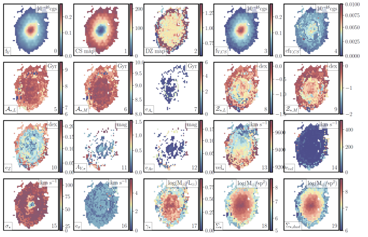
Fig. 2 Example of the content of the SSP extension in the Pipe3D FITS file, corresponding to the galaxy CAVITY66239. Each panel shows a color image with the property stored in the corresponding channel of the data cube, including, from top-left to bottom-right: (i) the flux intensity in the pseudo V-band (f V ); (ii) the identification index of each voxel/texella at which each spaxel is assigned in the binning process (CS map); (iii) the dezonification map, i.e., the ratio between the flux intensity in the V-band at each particular pixel and the average flux intensity within the voxel to which this pixel is assigned (DZ map); (iv) flux-intensity in the V-band after binning the cube spatially (f V , CS ); (v) standard deviation of the flux-intensity along the wavelength considered to derive the pseudo V-band image, adopted as upper limit of the noise level (ef V , CS ); (vi) luminosity-weighted age (𝒜⋆, L ); (vii) mass-weighted age (𝒜⋆, M ); (viii) error estimated for the LW and MW ages (e𝒜⋆); (ix) luminosity-weighted metallicity (Z ⋆, L ); (x) mass-weighted metallicity (Z ⋆, M ); (xi) error estimated for the LW and MW metallicities (eZ ⋆); (xii) dust attenuation derived for the stellar populations (𝒜 V , ⋆); (xiii) error estimated for the dust attenuation (e𝒜 V , ⋆); (xiv) stellar velocity (vel⋆); (xv) error estimated for the stellar velocity (vel*); (xvi) stellar velocity dispersion (σ ⋆); (xvii) error estimated for the velocity dispersion (eσ; (xviii) average mass-to-light ratio (Υ ⋆); (xix) stellar mass density (Σ*); (xx) stellar mass density corrected by dust attenuation (Σ *,dust ). The index, corresponding property, and units, are indicated in each panel as a label at the bottom-right, bottom-left and top-right of the figure. The color figure can be viewed online.
SFH: Includes the spatial distribution of the coefficients w ⋆,L from the fitting of the stellar population with the templates from the adopted SSP library. The first 273 channels of the data cube cover the full spectrum of ages and metallicities (7) outlined in the MaStar_sLOG SSP template. Additionally, the cube includes 39 channels dedicated to the weights associated with each age (w ⋆,L (age)), calculated by summing all w ⋆,L across the seven metallicities for each age (channels 273 to 311). Moreover, there are 7 channels that capture the weights for each metallicity (w ⋆,L (met)), derived by aggregating all w ⋆,L for each metallicity across the 39 ages (channels 311 to 318). A description of the content of this extension is included in Table 3 in Sánchez et al. (2024a). Figure 3 visualizes the content of each extension by displaying the spatial distribution of age-related weights, w ⋆,L (age), organized into 10 age categories, for the galaxy CAVITY 66239.
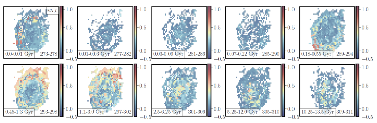
Fig. 3 Example of the content of the SFH extension in the Pipe3D fitsfile, corresponding to the galaxy CAVITY66239. Each panel shows a color image with the fraction of light at the normalization wavelength (w ⋆,L ) for different ranges of age included in the SSP library. The range of age is indicated in the bottom-left inbox, and the corresponding indices of the co-added channels in the SFH extension are shown in the bottom-right legend. For clarity we do not show the individual w ⋆,L maps included in the SFH extension. The color figure can be viewed online.
INDICES: Contains the spatial distribution of the stellar indices and their corresponding errors. A total of 33 indices is analyzed. A detailed description of the adopted wavelength to define the indices (and the adjacent continuum) and the procedures is given in detail in Lacerda et al. (2022) and in Sánchez et al. (2024a). An example of the content of this extension is included in Figure 4, showing the stellar indices derived for the galaxy CAVITY 66239.
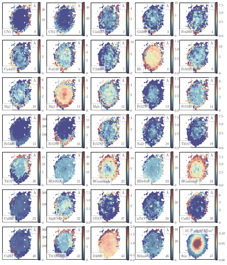
Fig. 4 Example of the content of the INDICES extension in the Pipe3D file, corresponding to the galaxy CAVITY66239. Each panel shows a color image with the content of a channel in this data cube. The actual content is indicated for each panel in the lower-left, the channel in the lower-right and the units of the represented quantity in the upper-right legend. The color figure can be viewed online.
ELINES: Comprises the properties of the strong emission lines derived by fitting them with a set of Gaussian functions (§ 4.1.3). The extension comprises the velocity and velocity dispersion maps for Hα (usually the strongest emission line in the considered wavelength range), and the flux intensities for the [O II], [O III] 4959,5007, Hβ, Hα, [N II] 6458,6583 [S II]6713,6717, and their corresponding errors. Figure 5 illustrates the content of this extension for the galaxy CAVITY 66239. We should stress that the velocity dispersion is provided in the observed units (Å), without subtracting the value of the instrumental resolution corresponding to the σ of the fitted Gaussian function.
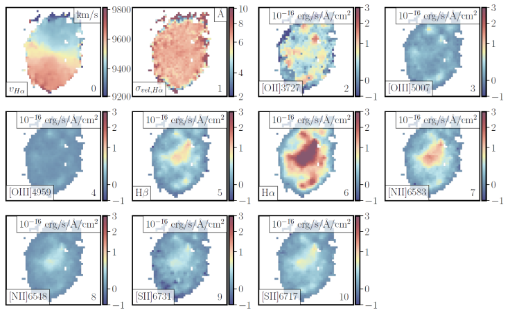
Fig. 5 Example of the content of the ELINES extension in the Pipe3D file, corresponding to the galaxy CAVITY66239. Each panel shows a color image with the content of a channel in this data cube. The 1st panel corresponds to the velocity, in km/s, and the 2nd panel to the velocity dispersion, in Å (to transform to km/s, it is required to subtract the instrumental dispersion). The remaining panels represent the distribution of the flux intensities for the different analyzed emission lines (lower-left legend). The color figure can be viewed online.
FLUX_ELINES and FLUX_ELINES_LONG: These contain the parameters of the emission lines derived using a weighted-moment analysis (§ 4.1.3), for two subsets of emission lines. The first case includes a list of 54 emission lines previously analyzed with Pipe3D for CALIFA data (Sánchez et al. 2016b). The second case uses a larger list of emission lines, with updated restframe wavelengths as included in Sánchez et al. (2022), adjusted for the narrower wavelength range of the current data (totaling 130 emission lines). The extension includes four distinct parameters: flux intensity, velocity, velocity dispersion, and equivalent width, along with their corresponding errors. Therefore, there are eight channels designated from I to I + 7N for the N different parameters calculated for the same I emission line. Here, 0 ≤ N < 8 and I ranges from 0 to 53 (for the FLUX_ELINES extension) or up to 130 (for the FLUX_ELINES_LONG extension). Figure 6 provides an illustration of what these extensions encompass, showcasing the four parameters determined for the Hα emission line, along with their respective errors, within the FLUX_ELINES extension, for the galaxy CAVITY 66239. Like in the case of the ELINES extension, the velocity dispersion is provided in the observed units (Å), without subtracting the value corresponding to the instrumental resolution. In the case of the FLUX_ELINES and FLUX_ELINES_LONG the reported quantity corresponds to the FWHM.
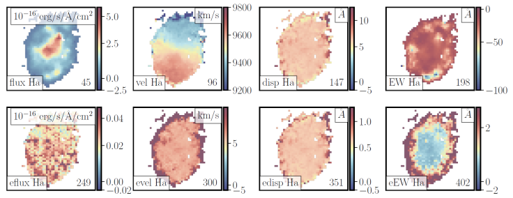
Fig. 6 Example of the content of the FLUX_ELINES extension in the Pipe3D file, corresponding to the galaxy CAVITY66239 for one particular emission line (Hα). From top-left to bottom-right the figure shows the flux intensity [10−16 erg/s/Å/cm2], the velocity [km/s], the velocity dispersion, FWHM [Å], the EW Hα [Å], and the corresponding errors. The color figure can be viewed online.
GAIA_MASK: A mask of field stars derived from the Gaia catalog as described in § 4.2.
SELECT_REG: A mask of regions with a signal-to-noise ratio greater than 3 in the stellar continuum (V-band), i.e., areas where the analysis of the stellar population is considered reliable.
TABLE 1 DESCRIPTION OF THE PIPE3D FILE
| HDU | EXTENSION | Dimensions |
|---|---|---|
| 0 | ORG_HDR | () |
| 1 | SSP | (NX, NY, 25) |
| 2 | SFH | (NX, NY, 319) |
| 3 | INDICES | (NX, NY, 70) |
| 4 | ELINES | (NX, NY, 11) |
| 5 | FLUX_ELINES | (NX, NY, 432) |
| 6 | FLUX_ELINES_LONG | (NX, NY, 1040) |
| 7 | GAIA_MASK | (NX, NY) |
| 8 | SELECT_REG | (NX, NY) |
For each analyzed galaxy (CUBENAME.V500.rscube.fits.gz), we provide one of these files, adopting the nomenclature CUBENAME.Pipe3D.cube.fits.gz.
5.2. Catalog of Individual Parameters
As outlined in § 4.4, guided by the methodologies of Sánchez et al. (2022, 2024a), we calculate a variety of specific parameters for each galaxy. These encompass integrated and aperture-limited values, as well as characteristic parameters (such as those at the effective radius). Additionally, for some parameters, we also determine the slopes of their radial gradients. This process utilizes the data contained within each individual pyPipe3D file, as detailed in § 5.1, and employs the calculation methods described in Sánchez et al. (2024a). The final catalog, included in the CAVITY.pyPipe3D.fits FITs file, comprises 559 parameters. Table 2 lists the first 5 of them; the details of the remaining parameters were already included in Table 2 of Sánchez et al. (2024a). We include here just the first rows that contain the only differences between both tables to avoid repetition. Nevertheless an electronic format of the description of the complete table is provided in the CALIFA 1st DR web page.
TABLE 2 INTEGRATED AND CHARACTERISTIC PARAMETERS FOR EACH DATA CUBE
| # | Param | Units | Description |
|---|---|---|---|
| 0 | ID | - | Running index |
| 1 | cubename | - | CAVITY galaxy (cube) name |
| 2 | ra | deg | Right Ascension of the object |
| 3 | dec | deg | Declination of the object |
| 4 | void | - | Void location of the galaxy |
| 5 | TType | - | Hubble Type number |
| ... | ... | ... | ... |
For the remaining parameters we refer the reader to Table 2 of Sánchez et al. (2024a).
5.3. The Relations that Rule SF
An example of the use of the content of the delivered data products to explore the global extensive and intensive relations that rule star-formation (SF) in galaxies (Sánchez 2020, for a review on the topic).
5.3.1. A Brief Introduction to the SF Scaling Relations
Schmidt (1959) initially proposed a theoretical relation between the star formation rate (SFR) and the gas density within a specific volume. This relation was further examined in Schmidt (1968), but it wasn’t until Kennicutt (1998b) that it was articulated in its modern form: a log-log (or power-law) relationship between the SFR surface density (ΣSFR) and the gas surface density (Σgas), representing two intensive parameters independent of galaxy size. Kennicutt (1998a) predicted a slope of approximately 1.4 for this relationship, based on considerations of the free-fall time for a self-collapsing cloud. While originally derived for global intensive parameters, it is now understood to be applicable above the typical scale of large molecular clouds (≈ 500 pc), characterizing spatially resolved sub-galactic structures as well (e.g., the rSK-law; Wong & Blitz 2002; Kennicutt et al. 2007). Both the global and resolved relations exhibit a similar dispersion, around ≈ 0.2 dex (Bigiel et al. 2008; Leroy et al. 2013). However, discrepancies in the slope have been observed when compared to theoretical predictions, with contemporary estimations leaning towards a slope of ≈ 1 (e.g., Sánchez 2020; Sánchez et al. 2021b).
The relationship between SFR and M⋆ has been more recently uncovered, following analyses of extensive galaxy surveys like the Sloan Digital Sky Survey (SDSS; York et al. (2000)). Known as the star-formation main sequence (SFMS), this tight correlation (dispersion ≈ 0.25 dex) between the logarithms of these two quantities, with a slope close to one, is observed exclusively in star-forming galaxies, where ionization is predominantly influenced by young, massive OB stars. It has been detected across a broad spectrum of redshifts in detail particularly in the nearby Universe (z ≈ 0), but is evident up to redshifts of 1-2 (e.g., Speagle et al. (2014), Rodríguez-Puebla et al. (2016)). The relation demonstrates noticeable evolution, particularly in its zero-point, reflecting the increase in stellar masses and decrease in SFR from early cosmological times to the present. Two nearly simultaneous studies, Sánchez et al. (2013) and Wuyts et al. (2013), introduced the concept of a resolved version of this relation, applicable down to ≈ kpc scales, the rSFMS, noted for its tight correlation between the logarithms of ΣSFR and Σ*. Further investigations, such as that by Cano-Díaz et al. (2016a), utilizing data from the CALIFA survey (Sánchez et al. 2012), have definitively established its characteristics and form. The potential dependency of this relation on other galactic properties, like morphology, has been probed by various authors, (e.g., González Delgado et al. 2016; Catalán-Torrecilla et al. 2017; Cano-Díaz et al. 2019; Méndez-Abreu et al. 2019).
A third correlation, this time between molecular gas and stellar masses in star-forming galaxies (SFGs), has also been delineated (e.g. Saintonge et al. 2016; Calette et al. 2018). Similar to the preceding two, this relationship, dubbed the molecular gas main sequence (MGMS), features a tight correlation with a slope close to one. Its resolved counterpart at the kiloparsec scale, the rMGMS, has been explored more recently (Lin et al. 2019), relating the corresponding intensive parameters: Σgas versus Σ*, using a combination of IFS data from the MaNGA survey (Bundy et al. 2015) and CO mapping from the ALMAQUEST compilation (Lin et al. 2020).
Bolatto et al. (2017) first demonstrated that a simple parametrization of the global intensive Schmidt-Kennicutt relation mirrors the distribution observed in the resolved rSK between ΣSFR and Σgas. Subsequent detailed studies have confirmed this correspondence between the global extensive SFMS and the local/resolved rSFMS (Pan et al. 2018; Cano-Díaz et al. 2019). Finally, it has been established that the global intensive relations (where ΣSFR, Σgas, and Σ* are measured as average quantities galaxy-wide) and the local/resolved relations (where these parameters are measured in star-forming regions at a kpc-scale) exhibit the same distributions, slopes, and similar zero points (e.g. Sánchez et al. 2021b,a, 2023c).
5.3.2. Selecting SF-Galaxies Using the WHaD Diagram
We explore here those relations for the analyzed CAVITY sub-sample. To do so we first need to select the star-forming galaxies among them. We depart from the classical approach, frequently adopted in the literature, that uses the classical diagnostic-diagrams that compare pairs of collisionally excited versus Balmer photoionized emission lines (e.g., the BPT diagram that compares [O III]/Hβ vs. [N II]/Hα, Baldwin et al. 1981). Instead, we select the SF galaxies using the recently introduced WHaD diagram, that makes use of the EW and the velocity dispersion of a single emission line, Hα (Sánchez et al. 2024). In this way we illustrate the quality (and useability) of the kinematics analysis performed by pyPipe3D.
Following Sánchez (2020); Sánchez et al. (2021b), we consider that a galaxy is actively forming stars if its ionization is dominated by OB-stars at the effective radius, assuming that the values at this galactocentric distance are characteristic of the average properties in a galaxy (González Delgado et al. 2014, 2015). In this way, we extract the following parameters from the delivered catalog, all estimated at 1 effective radius: (i) the flux intensities of [O III], Hβ, [N II] and Hα; (ii) the EW(Hα), and (iii) the velocity dispersion of Ha (σ Hα ).
Figure 7 shows the distribution of the analyzed galaxies in the WHaD diagram, color-coded by the [N ii]/Hα line ratio. As expected, due to the predominance of late-type (Sc) galaxies in the CAVITY observed sample, most of the galaxies are located in the region associated with star-formation in this diagram. This region corresponds to galaxies with an EW(Hα)>3Å and a σ Hα >57 km s−1, comprising a total of 122 galaxies. These are the SF galaxies (SFGs) that we will use to explore the relations described in the previous section. It can be noticed that most of them present low-values of [N II]/Hα. On the contrary, outside this region, in areas of the WHaD diagram assigned to ionizations due to strong or weak AGNs, the galaxies present larger values of this line ratio, in agreement with the expectations using other more classical diagnostic diagrams such as the WHaN diagram (Cid Fernandes et al. 2010) or the already mentioned BPT diagram. This is illustrated in Figure 7, right panels, which showns the distribution of the full sample (central panel) and SF-sub-sample (right panel) in the BPT diagram. It is evident that the galaxies selected using the WHaD diagram are found in the classical location of HII-regions, dominated by photoinization by OB-stars (e.g. Osterbrock 1989). After applying these criteria we end up with 122 star forming galaxies out of the 208 galaxies analysed.
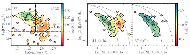
Fig. 7 Diagnostic-diagrams for the analyzed CAVITY sample using emission line values estimated at one effective radius. Left-panel: WHaD diagram (σ Hα vs. EW(Hα)) for the full sample. Right-panels: BPT diagram ([O III]/Hβ vs. [N II]/Hα, Baldwin et al. 1981), for the full sample (left) and the SF sub-sample selected using the WHaD diagram (right). In each panel contours represent the density points (encircling 5%, 45% and 85% of the points, respectively), and colors represent the average value of a particular emission line property: [N II]/Hα, in the WHaD diagram, and EW(Hα), in the BPT diagrams. The dashed line in the WHaD diagram represents the boundaries between different ionizations proposed for this diagram, with the different ionizations labeled in each regime. The dotted and dash-dotted lines in the BPT diagram correspond to the demarcation lines usually adopted to distinguish between SF and AGNs, proposed by Kauffmann et al. (2003) and Kewley et al. (2001), respectively. The color figure can be viewed online.
5.3.3. Extensive and Intensive Scaling Relations
Once the SFGs were selected, we followed the methodology outlined by Cano-Díaz et al. (2019) to examine the global extensive relationships among the three extracted parameters (SFR, M ∗, and M gas), analyzing the distribution and relationship between SFR-M ∗ (SFMS), M gas-M ∗ (MGMS), and SFR-M gas (SK). Those parameters were derived as described in § 4.3 and are included in the catalog described in § 5.2. Figure 8, top panels, displays these distributions for the selected SFGs, which show clear linear trends in all three cases, delineating the well-established relations. To parameterize these relationships, we employ a binning strategy on the x-axis and y-axis data, calculating the mean and standard deviation within bins of 0.25 dex. From these two bins the code selects the values that are closer to the peak density. The locations of the final binned data are also illustrated in the respective panels. Subsequently, we conducted a simple linear regression on the binned data to ascertain the best-fitting relation between each pair of parameters. Error estimations were obtained through a Monte-Carlo iteration applied to the original data set, thereby facilitating the propagation of errors for each derived parameter.
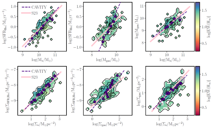
Fig. 8 Global/Integrated extensive (top-panels) and intensive (bottom-panels) relations that rule SF in galaxies. From top-left to bottom-right is shown the distribution of (i) SFR vs. M*, (ii) SFR vs. M gas , (iii) M gas vs. M*, (iv) ΣSFR vs. Σ*, (v) ΣSFR vs. Σ gas and (vi) Σ gas vs. Σ*. In each panel contours represent the density points (encircling 5%, 45% and 85% of the points, respectively), and colors represent the average value of EW(Hα)$. We adopted the same scale range used in Figure 7, to clearly see that all selected galaxies are indeed SFGs. Finally, dark purple circles correspond to a binning that traces the peaks of the density. The dark purple dashed-line represents the best linear relation for the binned values (labelled as CAVITY), and the pink solid line corresponds to the values reported by Sánchez et al. (2023c) (labelled as S23). The color figure can be viewed online.
Table 3 show the results of this analysis, including the zero-point (β) and slope (α) of the three relations, with their corresponding errors, together with the correlation coefficient (r c), and the standard deviation of the dependent parameter before (σ obs) and after applying the best fitted linear relation (σ exp). In all instances, the slopes approximate unity, being compatible within approximately 1σ with this value. The Schmidt-Kennicutt law (SK-law) exhibits the most significant deviation from this norm.
TABLE 3 RESULTS OF THE ANALYSIS OF GLOBAL SF-RELATIONS
| Relation | β | α | r c | σ obs | σ exp |
|---|---|---|---|---|---|
| SFMS | -9.38±1.36 | 0.92±0.39 | 0.73 | 0.25 | 0.17 |
| SK | -11.88±1.40 | 1.26±0.46 | 0.66 | 0.26 | 0.16 |
| MGMS | -1.97±1.62 | 1.12±0.63 | 0.66 | 0.25 | 0.18 |
| rSFMS | -10.13±0.59 | 0.97±0.41 | 0.82 | 0.31 | 0.18 |
| rSK | -9.50±0.50 | 1.02±0.45 | 0.72 | 0.31 | 0.26 |
| rMGMS | -0.81±0.43 | 1.05±0.32 | 0.62 | 0.35 | 0.28 |
Zero-point (β) and slope (α) of the three extensive global relations (SFMS, SK and MGMS), and the corresponding intensive ones (rSFMS, rSK, rMGMS) shown in Figure 8. In addition, we include the correlation coefficient (r c), the standard deviation of the distribution of data before (σ obs) and after applying the best fitted linear relation (σ exp).
Following the derivation of the extensive relations, we conducted a
subsequent analysis focusing on the global intensive relations
(ΣSFR, Σ∗, and Σgas). To calculate
these parameters, we adhered to the methodology outlined by Sánchez et al. (2021b) and Sánchez et al. (2023c), involving the
division of the respective extensive parameter by the effective area
encompassed by each galaxy (defined as
Despite the limited number of galaxies explored in this analysis (≈122 SF-galaxies), and the smaller range of stellar masses sampled, current results agree with the most recent explorations on the topic. For instance, the compilation of values reported by Sánchez et al. (2023c) indicates that the slope of the different global intensive relations covers a range of values of (i) 0.74-1.02 (rSFMS), (ii) 0.76-0.98 (rSK) and (iii) 0.73-1.15 (rMGMS), with a typical error of ≈0.11-0.27. Indeed, the zero-points and slopes estimated for the intensive relations match better the values reported in the literature than those estimated for the extensive relation, as appreciated in the comparison included in Figure 8 (in particular for the SK-relation). That is also expected as the dynamical range of the extensive quantities in the observed CAVITY sample is shorter than that covered by other less focused surveys (see Figure 1, for instance), and the derivation of this kind of extensive relation is less accurate. Furthermore, the values reported for the slopes and zero-points are also compatible with the corresponding resolved intensive relations (see Sánchez et al. 2023c, Table 1), in agreement with the results presented by Sánchez et al. (2021a).
6. Summary and conclusions
Throughout this article, we present the spatially resolved spectroscopic properties of galaxies obtained using integral field spectroscopy (IFS) data for the currently observed CAVITY project. When compared with the most recent distributions of similar products, such as the results from the analysis using pyPipe3D on the final data release (DR) of the MaNGA IFS galaxy survey (Sánchez et al. 2022) or the eCALIFA survey (Sánchez et al. 2024a), we recognize that both distributions encompass a much larger number of galaxies (≈ 10,000 and ≈900, respectively). However, none of the surveys sample galaxies directly selected to be located in voids. Therefore, while they may be representative of the bulk population, they lack the ability to determine the potential differences in the evolution and properties of galaxies in these low populated regions of the Universe.
This article details the analysis conducted on this data set. For each galaxy, we provide a single FITS file containing different extensions, each of which includes the spatial distributions of various physical and observational quantities derived from the analysis. We offer a detailed description of each of these extensions, exemplifying their content with the results for the galaxy CAVITY 66239 as a case study. Additionally, we extract a set of integrated and/or characteristic parameters for each galaxy and, when necessary, the slopes of their radial gradients. In this way, a catalog containing over 550 derived quantities for each object in the dataset is also provided. The delivered data set is restricted to the galaxies distributed in the 1st CAVITY data release, and would be incremented in successive distributions along the lifetime of the survey.
The utility of this new set of data products is demonstrated using as examples the global extensive and intensive relations that rule SF galaxy wide, i.e., the (r)SFMS, (r)SK and (r)MGMS relations. To do so we select SFGs using the recently presented WHaD diagram, a novelty that allows us to illustrate the quality of our analysis, not only to recover the flux intensities of the emission lines but also their kinematics properties. Once the SFGs is selected, we examine the described relation characterizing them with a linear relation (between the logarithm of the involved quantities). We find a remarkable agreement with the most recent results in the literature, in particular for the global intensive relations, that exhibit similar shape (slope), strength (correlation coefficients) and tightness (dispersion of the residuals), despite the fact of the nature of the sample (void galaxies) and its limited number (≈122 SFGs).
The comprehensive suite of data products and the catalog of individual quantities are freely available for community use as part of the CAVITY data release for the subset of analyzed galaxies part of the CAVITY DR1.
This research made use of Astropy,13 a community-developed core Python package for Astronomy (Astropy Collaboration et al. 2013, 2018).

